class: center, middle, inverse, title-slide # An Introduction: R + the <code>tidyverse</code> ## For Dr. Abner’s Public Management Course <html> <div style="float:left"> </div> <hr color='#e2f1fc' size=1px width=1100px> </html> ### <span style="color:#005f86; font-weight:500">Matt Worthington</span> | Sr. Project Manager for Data Initiatives, UT Austin - LBJ ### <span style="color:#bf5700; font-weight:300">September 13, 2021</span> --- background-image: url('assets/images/analysis_screen1.png') background-size: cover <style>.shareagain-bar { --shareagain-foreground: rgb(255, 255, 255); --shareagain-background: rgba(0, 0, 0, 0.5); --shareagain-facebook: none; --shareagain-pinterest: none; --shareagain-reddit: none; }</style> --- class: middle, center <img src="intro_slides_files/figure-html/unnamed-chunk-2-1.png" width="1008" /> --- background-image: url('assets/images/dir_stat.png') background-size: cover class: center, bottom, inverse --- class: middle .pull-left[ # About Me ] .pull-right[ * .orange[**Personal Background**]: Born and raised in San Antonio, Texas. Live in Austin with my wife and three kids. * .orange[**Education Backgrounds**]: English Studies, Special Education, and Public Policy * .orange[**Professional Backgrounds**]: Public School Teacher, School District Administrator, and Data Scientist. ] --- background-image: url('https://utexas-lbjp-data.github.io/assets/rmarkdown/slide_02.jpeg') background-size: cover class: center, bottom, inverse --- background-image: url('https://utexas-lbjp-data.github.io/assets/rmarkdown/slide_03.jpeg') background-size: cover class: center, bottom, inverse --- background-image: url('assets/images/hermione_spell_class.png') background-size: cover class: center, bottom, inverse ## .blue[How to understand R if you are new...] --- background-image: url('assets/images/hp_vs_r.png') background-size: cover class: center, bottom, inverse --- # How I Hope We End Today .pull-left[ #### Anywhere from here.. .rmd-img[] ] .pull-right[ #### to here. .rmd-img[] ] --- class: showcase-bg, section, center, middle # 🪄 Showcase --- # Census Spellbook: `tidycensus` .pull-left[ ```r library(tidycensus) # Create A List of Variables demvars <- c(White = "P005003", Black = "P005004", Asian = "P005006", Hispanic = "P004003") # Pull The Census Data harris <- get_decennial( geography = "tract", variables = demvars, state = "TX", county = "Harris County", geometry = TRUE, summary_var = "P001001" ) |> # Create pct column mutate(pct = 100 * (value / summary_value)) # Draw A Chart harris |> ggplot(aes(fill = pct)) + facet_wrap(~variable) + geom_sf(color = NA) + coord_sf(crs = 26915, datum=NA) + scale_fill_viridis_c() + theme_lbj() + labs(title="Population Demographics in Harris County", subtitle="US Census | 2010 Decennial Census") ``` ] .pull-right[ <img src="intro_slides_files/figure-html/unnamed-chunk-5-1.png" width="504" /> ] --- # Table Spellbook: `gt` .pull-left[ ```r library(gt) # Create A List of Variables demvars <- c(White = "P005003", Black = "P005004", Asian = "P005006", Hispanic = "P004003", AIAN = "P005005", NHOPI = "P005007", Other = "P003007",`Two or More` = "P003008") # Pull The Census Data harris <- get_decennial(geography = "county", variables = demvars, state = "TX", county = "Harris County", summary_var = "P001001") |> # Create pct column mutate(pct = (value / summary_value)) |> select(variable, value, pct) # Draw A Table harris |> gt() |> # Pass The Data To A gt table tab_header(title = md("**Demographics in Harris County**"), subtitle = "Harris County reported 4,092,459 residents in the 2010 Census. Here's how each demographic group compares to the total population.") |> tab_source_note(source_note = "Data: US Census | 2010 Decennial Census | pulled with {tidycensus} in R") |> fmt_number(columns = c("value")) |> fmt_percent(columns = c("pct")) |> cols_label( variable = md("**Group**"), value = md("**Population**"), pct = md("**Pct. of Total**") ) ``` ] .pull-right[ <div id="wxnizxjmbl" style="overflow-x:auto;overflow-y:auto;width:auto;height:auto;"> <style>html { font-family: -apple-system, BlinkMacSystemFont, 'Segoe UI', Roboto, Oxygen, Ubuntu, Cantarell, 'Helvetica Neue', 'Fira Sans', 'Droid Sans', Arial, sans-serif; } #wxnizxjmbl .gt_table { display: table; border-collapse: collapse; margin-left: auto; margin-right: auto; color: #333333; font-size: 16px; font-weight: normal; font-style: normal; background-color: #FFFFFF; width: auto; border-top-style: solid; border-top-width: 2px; border-top-color: #A8A8A8; border-right-style: none; border-right-width: 2px; border-right-color: #D3D3D3; border-bottom-style: solid; border-bottom-width: 2px; border-bottom-color: #A8A8A8; border-left-style: none; border-left-width: 2px; border-left-color: #D3D3D3; } #wxnizxjmbl .gt_heading { background-color: #FFFFFF; text-align: center; border-bottom-color: #FFFFFF; border-left-style: none; border-left-width: 1px; border-left-color: #D3D3D3; border-right-style: none; border-right-width: 1px; border-right-color: #D3D3D3; } #wxnizxjmbl .gt_title { color: #333333; font-size: 125%; font-weight: initial; padding-top: 4px; padding-bottom: 4px; border-bottom-color: #FFFFFF; border-bottom-width: 0; } #wxnizxjmbl .gt_subtitle { color: #333333; font-size: 85%; font-weight: initial; padding-top: 0; padding-bottom: 6px; border-top-color: #FFFFFF; border-top-width: 0; } #wxnizxjmbl .gt_bottom_border { border-bottom-style: solid; border-bottom-width: 2px; border-bottom-color: #D3D3D3; } #wxnizxjmbl .gt_col_headings { border-top-style: solid; border-top-width: 2px; border-top-color: #D3D3D3; border-bottom-style: solid; border-bottom-width: 2px; border-bottom-color: #D3D3D3; border-left-style: none; border-left-width: 1px; border-left-color: #D3D3D3; border-right-style: none; border-right-width: 1px; border-right-color: #D3D3D3; } #wxnizxjmbl .gt_col_heading { color: #333333; background-color: #FFFFFF; font-size: 100%; font-weight: normal; text-transform: inherit; border-left-style: none; border-left-width: 1px; border-left-color: #D3D3D3; border-right-style: none; border-right-width: 1px; border-right-color: #D3D3D3; vertical-align: bottom; padding-top: 5px; padding-bottom: 6px; padding-left: 5px; padding-right: 5px; overflow-x: hidden; } #wxnizxjmbl .gt_column_spanner_outer { color: #333333; background-color: #FFFFFF; font-size: 100%; font-weight: normal; text-transform: inherit; padding-top: 0; padding-bottom: 0; padding-left: 4px; padding-right: 4px; } #wxnizxjmbl .gt_column_spanner_outer:first-child { padding-left: 0; } #wxnizxjmbl .gt_column_spanner_outer:last-child { padding-right: 0; } #wxnizxjmbl .gt_column_spanner { border-bottom-style: solid; border-bottom-width: 2px; border-bottom-color: #D3D3D3; vertical-align: bottom; padding-top: 5px; padding-bottom: 5px; overflow-x: hidden; display: inline-block; width: 100%; } #wxnizxjmbl .gt_group_heading { padding: 8px; color: #333333; background-color: #FFFFFF; font-size: 100%; font-weight: initial; text-transform: inherit; border-top-style: solid; border-top-width: 2px; border-top-color: #D3D3D3; border-bottom-style: solid; border-bottom-width: 2px; border-bottom-color: #D3D3D3; border-left-style: none; border-left-width: 1px; border-left-color: #D3D3D3; border-right-style: none; border-right-width: 1px; border-right-color: #D3D3D3; vertical-align: middle; } #wxnizxjmbl .gt_empty_group_heading { padding: 0.5px; color: #333333; background-color: #FFFFFF; font-size: 100%; font-weight: initial; border-top-style: solid; border-top-width: 2px; border-top-color: #D3D3D3; border-bottom-style: solid; border-bottom-width: 2px; border-bottom-color: #D3D3D3; vertical-align: middle; } #wxnizxjmbl .gt_from_md > :first-child { margin-top: 0; } #wxnizxjmbl .gt_from_md > :last-child { margin-bottom: 0; } #wxnizxjmbl .gt_row { padding-top: 8px; padding-bottom: 8px; padding-left: 5px; padding-right: 5px; margin: 10px; border-top-style: solid; border-top-width: 1px; border-top-color: #D3D3D3; border-left-style: none; border-left-width: 1px; border-left-color: #D3D3D3; border-right-style: none; border-right-width: 1px; border-right-color: #D3D3D3; vertical-align: middle; overflow-x: hidden; } #wxnizxjmbl .gt_stub { color: #333333; background-color: #FFFFFF; font-size: 100%; font-weight: initial; text-transform: inherit; border-right-style: solid; border-right-width: 2px; border-right-color: #D3D3D3; padding-left: 12px; } #wxnizxjmbl .gt_summary_row { color: #333333; background-color: #FFFFFF; text-transform: inherit; padding-top: 8px; padding-bottom: 8px; padding-left: 5px; padding-right: 5px; } #wxnizxjmbl .gt_first_summary_row { padding-top: 8px; padding-bottom: 8px; padding-left: 5px; padding-right: 5px; border-top-style: solid; border-top-width: 2px; border-top-color: #D3D3D3; } #wxnizxjmbl .gt_grand_summary_row { color: #333333; background-color: #FFFFFF; text-transform: inherit; padding-top: 8px; padding-bottom: 8px; padding-left: 5px; padding-right: 5px; } #wxnizxjmbl .gt_first_grand_summary_row { padding-top: 8px; padding-bottom: 8px; padding-left: 5px; padding-right: 5px; border-top-style: double; border-top-width: 6px; border-top-color: #D3D3D3; } #wxnizxjmbl .gt_striped { background-color: rgba(128, 128, 128, 0.05); } #wxnizxjmbl .gt_table_body { border-top-style: solid; border-top-width: 2px; border-top-color: #D3D3D3; border-bottom-style: solid; border-bottom-width: 2px; border-bottom-color: #D3D3D3; } #wxnizxjmbl .gt_footnotes { color: #333333; background-color: #FFFFFF; border-bottom-style: none; border-bottom-width: 2px; border-bottom-color: #D3D3D3; border-left-style: none; border-left-width: 2px; border-left-color: #D3D3D3; border-right-style: none; border-right-width: 2px; border-right-color: #D3D3D3; } #wxnizxjmbl .gt_footnote { margin: 0px; font-size: 90%; padding: 4px; } #wxnizxjmbl .gt_sourcenotes { color: #333333; background-color: #FFFFFF; border-bottom-style: none; border-bottom-width: 2px; border-bottom-color: #D3D3D3; border-left-style: none; border-left-width: 2px; border-left-color: #D3D3D3; border-right-style: none; border-right-width: 2px; border-right-color: #D3D3D3; } #wxnizxjmbl .gt_sourcenote { font-size: 90%; padding: 4px; } #wxnizxjmbl .gt_left { text-align: left; } #wxnizxjmbl .gt_center { text-align: center; } #wxnizxjmbl .gt_right { text-align: right; font-variant-numeric: tabular-nums; } #wxnizxjmbl .gt_font_normal { font-weight: normal; } #wxnizxjmbl .gt_font_bold { font-weight: bold; } #wxnizxjmbl .gt_font_italic { font-style: italic; } #wxnizxjmbl .gt_super { font-size: 65%; } #wxnizxjmbl .gt_footnote_marks { font-style: italic; font-weight: normal; font-size: 65%; } </style> <table class="gt_table"> <thead class="gt_header"> <tr> <th colspan="3" class="gt_heading gt_title gt_font_normal" style><strong>Demographics in Harris County</strong></th> </tr> <tr> <th colspan="3" class="gt_heading gt_subtitle gt_font_normal gt_bottom_border" style>Harris County reported 4,092,459 residents in the 2010 Census. Here's how each demographic group compares to the total population.</th> </tr> </thead> <thead class="gt_col_headings"> <tr> <th class="gt_col_heading gt_columns_bottom_border gt_left" rowspan="1" colspan="1"><strong>Group</strong></th> <th class="gt_col_heading gt_columns_bottom_border gt_right" rowspan="1" colspan="1"><strong>Population</strong></th> <th class="gt_col_heading gt_columns_bottom_border gt_right" rowspan="1" colspan="1"><strong>Pct. of Total</strong></th> </tr> </thead> <tbody class="gt_table_body"> <tr><td class="gt_row gt_left">White</td> <td class="gt_row gt_right">1,349,646.00</td> <td class="gt_row gt_right">32.98%</td></tr> <tr><td class="gt_row gt_left">Black</td> <td class="gt_row gt_right">754,258.00</td> <td class="gt_row gt_right">18.43%</td></tr> <tr><td class="gt_row gt_left">Asian</td> <td class="gt_row gt_right">249,853.00</td> <td class="gt_row gt_right">6.11%</td></tr> <tr><td class="gt_row gt_left">Hispanic</td> <td class="gt_row gt_right">1,671,540.00</td> <td class="gt_row gt_right">40.84%</td></tr> <tr><td class="gt_row gt_left">AIAN</td> <td class="gt_row gt_right">8,150.00</td> <td class="gt_row gt_right">0.20%</td></tr> <tr><td class="gt_row gt_left">NHOPI</td> <td class="gt_row gt_right">2,260.00</td> <td class="gt_row gt_right">0.06%</td></tr> <tr><td class="gt_row gt_left">Other</td> <td class="gt_row gt_right">583,566.00</td> <td class="gt_row gt_right">14.26%</td></tr> <tr><td class="gt_row gt_left">Two or More</td> <td class="gt_row gt_right">131,332.00</td> <td class="gt_row gt_right">3.21%</td></tr> </tbody> <tfoot class="gt_sourcenotes"> <tr> <td class="gt_sourcenote" colspan="3">Data: US Census | 2010 Decennial Census (pulled with {tidycensus} in R)</td> </tr> </tfoot> </table> </div> ] --- # Static Charts: [`ggplot`]() .pull-left[  ] .pull-right[  ] --- # Interactive Charts: [`highcharter`](https://jkunst.com/highcharter/index.html) <div id="htmlwidget-f69d2ced27043bb4e630" style="width:100%;height:500px;" class="highchart html-widget"></div> <script type="application/json" data-for="htmlwidget-f69d2ced27043bb4e630">{"x":{"hc_opts":{"chart":{"reflow":true},"title":{"text":"Texas Effective Reproduction Rate · R<sub>t<\/sub>","useHTML":true},"yAxis":{"title":{"text":"Effective Reproduction Rate (R<sub>t<\/sub>)"},"type":"linear","min":0.709633704100224,"max":3.35636466891657},"credits":{"enabled":true,"text":"Source: rt.live Analysis","href":"https://rt.live"},"exporting":{"enabled":true,"scale":2,"sourceWidth":1200,"sourceHeight":600,"allowHTML":true,"buttons":{"contextButton":{"menuItems":["downloadCSV","downloadCSV","separator","downloadPNG","downloadJPEG","downloadPDF"],"symbol":"menuball","symbolStrokeWidth":1,"symbolFill":"rgba(255,209, 0, 0.9)","symbolStroke":"#3A4A9F","theme":{"fill":"#fff"}}},"chartOptions":{"title":{"style":{"fontWeight":"800","fontSize":"22px","textTransform":"uppercase"}},"subtitle":{"style":{"fontSize":"14px"}}}},"boost":{"enabled":false},"plotOptions":{"series":{"label":{"enabled":false},"turboThreshold":0,"showInLegend":false},"treemap":{"layoutAlgorithm":"squarified"},"scatter":{"marker":{"symbol":"circle"}},"arearange":{"fillOpacity":0.3}},"series":[{"group":"group","data":[{"date":"2020-02-25","region":"TX","index":0,"mean":2.96292831028204,"median":2.94383875070423,"lower_80":2.52970475837423,"upper_80":3.35636466891657,"infections":28.9018806540979,"test_adjusted_positive":0,"test_adjusted_positive_raw":0,"positive":0,"tests":0,"new_tests":null,"new_cases":null,"new_deaths":null,"x":1582588800000,"y":2.96292831028204},{"date":"2020-02-26","region":"TX","index":1,"mean":2.97041387930373,"median":2.95543480434845,"lower_80":2.55749725490925,"upper_80":3.33399299771378,"infections":0.612634227650061,"test_adjusted_positive":0,"test_adjusted_positive_raw":0,"positive":0,"tests":0,"new_tests":null,"new_cases":null,"new_deaths":null,"x":1582675200000,"y":2.97041387930373},{"date":"2020-02-27","region":"TX","index":2,"mean":2.97127501616663,"median":2.95905410665407,"lower_80":2.5879885308644,"upper_80":3.32577043215825,"infections":8.69264110116989,"test_adjusted_positive":0,"test_adjusted_positive_raw":0,"positive":0,"tests":0,"new_tests":null,"new_cases":null,"new_deaths":null,"x":1582761600000,"y":2.97127501616663},{"date":"2020-02-28","region":"TX","index":3,"mean":2.97012509161931,"median":2.95045986799283,"lower_80":2.61494281042498,"upper_80":3.32992474209759,"infections":16.6804807584935,"test_adjusted_positive":0,"test_adjusted_positive_raw":0,"positive":0,"tests":0,"new_tests":null,"new_cases":null,"new_deaths":null,"x":1582848000000,"y":2.97012509161931},{"date":"2020-02-29","region":"TX","index":4,"mean":2.9749669690304,"median":2.95861541724178,"lower_80":2.56618946102579,"upper_80":3.27497593720589,"infections":19.5516401193951,"test_adjusted_positive":0,"test_adjusted_positive_raw":0,"positive":0,"tests":0,"new_tests":null,"new_cases":null,"new_deaths":null,"x":1582934400000,"y":2.9749669690304},{"date":"2020-03-01","region":"TX","index":5,"mean":2.97918558325031,"median":2.97448665012865,"lower_80":2.64028320643384,"upper_80":3.32005842802008,"infections":23.5948646387913,"test_adjusted_positive":0,"test_adjusted_positive_raw":0,"positive":0,"tests":0,"new_tests":null,"new_cases":null,"new_deaths":null,"x":1583020800000,"y":2.97918558325031},{"date":"2020-03-02","region":"TX","index":6,"mean":2.98293611629789,"median":2.9680134013894,"lower_80":2.65388599954327,"upper_80":3.29198534120647,"infections":30.3944123587228,"test_adjusted_positive":1.91906015783676,"test_adjusted_positive_raw":0,"positive":0,"tests":0,"new_tests":null,"new_cases":null,"new_deaths":null,"x":1583107200000,"y":2.98293611629789},{"date":"2020-03-03","region":"TX","index":7,"mean":2.97519265275669,"median":2.97033172398995,"lower_80":2.66136382993845,"upper_80":3.25998934956065,"infections":38.9800516503788,"test_adjusted_positive":3.00400720099162,"test_adjusted_positive_raw":0,"positive":0,"tests":0,"new_tests":0,"new_cases":0,"new_deaths":0,"x":1583193600000,"y":2.97519265275669},{"date":"2020-03-04","region":"TX","index":8,"mean":2.97317208739503,"median":2.96081656374523,"lower_80":2.66638907346211,"upper_80":3.25019845660066,"infections":49.5932977357261,"test_adjusted_positive":3.96069750211187,"test_adjusted_positive_raw":0,"positive":0,"tests":0,"new_tests":14,"new_cases":0,"new_deaths":0,"x":1583280000000,"y":2.97317208739503},{"date":"2020-03-05","region":"TX","index":9,"mean":2.95799204135674,"median":2.94726294923747,"lower_80":2.67723263274901,"upper_80":3.22994034560675,"infections":63.1552900064758,"test_adjusted_positive":5.27372025754494,"test_adjusted_positive_raw":0,"positive":0,"tests":0,"new_tests":930,"new_cases":0,"new_deaths":0,"x":1583366400000,"y":2.95799204135674},{"date":"2020-03-06","region":"TX","index":10,"mean":2.93615774581628,"median":2.93399896290443,"lower_80":2.6446873238548,"upper_80":3.18321231287537,"infections":80.5079409042078,"test_adjusted_positive":7.09745118282289,"test_adjusted_positive_raw":18.7719697307544,"positive":5,"tests":1286,"new_tests":1286,"new_cases":5,"new_deaths":0,"x":1583452800000,"y":2.93615774581628},{"date":"2020-03-07","region":"TX","index":11,"mean":2.90918883275478,"median":2.91007165517711,"lower_80":2.65100139391313,"upper_80":3.16930956010768,"infections":102.532333647027,"test_adjusted_positive":9.1402909681521,"test_adjusted_positive_raw":0,"positive":0,"tests":24,"new_tests":24,"new_cases":0,"new_deaths":0,"x":1583539200000,"y":2.90918883275478},{"date":"2020-03-08","region":"TX","index":12,"mean":2.86716990906637,"median":2.86242847450332,"lower_80":2.61981809989847,"upper_80":3.09940762899932,"infections":130.347355748329,"test_adjusted_positive":11.9496701515201,"test_adjusted_positive_raw":0,"positive":0,"tests":8,"new_tests":8,"new_cases":0,"new_deaths":0,"x":1583625600000,"y":2.86716990906637},{"date":"2020-03-09","region":"TX","index":13,"mean":2.81834909714127,"median":2.81149353342463,"lower_80":2.60510795951105,"upper_80":3.0717474626036,"infections":165.345364086142,"test_adjusted_positive":15.1286123105113,"test_adjusted_positive_raw":26.2807576230562,"positive":7,"tests":18,"new_tests":18,"new_cases":7,"new_deaths":0,"x":1583712000000,"y":2.81834909714127},{"date":"2020-03-10","region":"TX","index":14,"mean":2.75217611883319,"median":2.75977937145045,"lower_80":2.50691381375851,"upper_80":2.96935476547045,"infections":209.060746601156,"test_adjusted_positive":19.3228160996593,"test_adjusted_positive_raw":11.2631818384527,"positive":3,"tests":50,"new_tests":50,"new_cases":3,"new_deaths":0,"x":1583798400000,"y":2.75217611883319},{"date":"2020-03-11","region":"TX","index":15,"mean":2.68142301675504,"median":2.67651868168612,"lower_80":2.42260575399427,"upper_80":2.87361954057378,"infections":263.198632940079,"test_adjusted_positive":24.8044159608638,"test_adjusted_positive_raw":11.2631818384527,"positive":3,"tests":135,"new_tests":135,"new_cases":3,"new_deaths":0,"x":1583884800000,"y":2.68142301675504},{"date":"2020-03-12","region":"TX","index":16,"mean":2.5930097679754,"median":2.5951873377822,"lower_80":2.40591881072681,"upper_80":2.81303845589935,"infections":329.517518214475,"test_adjusted_positive":31.525516157021,"test_adjusted_positive_raw":15.0175757846035,"positive":4,"tests":305,"new_tests":305,"new_cases":4,"new_deaths":0,"x":1583971200000,"y":2.5930097679754},{"date":"2020-03-13","region":"TX","index":17,"mean":2.49497412668125,"median":2.49592993222198,"lower_80":2.28540341220357,"upper_80":2.68649295725618,"infections":409.866447254815,"test_adjusted_positive":40.2040072470556,"test_adjusted_positive_raw":0,"positive":0,"tests":655,"new_tests":655,"new_cases":0,"new_deaths":0,"x":1584057600000,"y":2.49497412668125},{"date":"2020-03-14","region":"TX","index":18,"mean":2.38672949800574,"median":2.38711854557697,"lower_80":2.20922262285091,"upper_80":2.59187699556915,"infections":505.822345378952,"test_adjusted_positive":51.2180246290633,"test_adjusted_positive_raw":0,"positive":0,"tests":960,"new_tests":960,"new_cases":0,"new_deaths":0,"x":1584144000000,"y":2.38672949800574},{"date":"2020-03-15","region":"TX","index":19,"mean":2.28158279380128,"median":2.27810142243553,"lower_80":2.1188512220477,"upper_80":2.46497680895095,"infections":618.49512559017,"test_adjusted_positive":65.28671011509,"test_adjusted_positive_raw":127.64939416913,"positive":34,"tests":530,"new_tests":530,"new_cases":34,"new_deaths":0,"x":1584230400000,"y":2.28158279380128},{"date":"2020-03-16","region":"TX","index":20,"mean":2.16888980049221,"median":2.16767720911864,"lower_80":2.00158983329511,"upper_80":2.33031491973282,"infections":748.367348241759,"test_adjusted_positive":82.9016181879299,"test_adjusted_positive_raw":0,"positive":0,"tests":575,"new_tests":575,"new_cases":0,"new_deaths":0,"x":1584316800000,"y":2.16888980049221},{"date":"2020-03-17","region":"TX","index":21,"mean":2.06122428795553,"median":2.06166025816266,"lower_80":1.90049606730944,"upper_80":2.21468208035306,"infections":895.809842387672,"test_adjusted_positive":105.12646437743,"test_adjusted_positive_raw":26.2807576230562,"positive":7,"tests":2606,"new_tests":2606,"new_cases":7,"new_deaths":1,"x":1584403200000,"y":2.06122428795553},{"date":"2020-03-18","region":"TX","index":22,"mean":1.95101458879892,"median":1.9441177158315,"lower_80":1.80841384837151,"upper_80":2.07964188027293,"infections":1059.96359631042,"test_adjusted_positive":132.951931112506,"test_adjusted_positive_raw":71.3334849768668,"positive":19,"tests":3299,"new_tests":3299,"new_cases":19,"new_deaths":1,"x":1584489600000,"y":1.95101458879892},{"date":"2020-03-19","region":"TX","index":23,"mean":1.84598031238549,"median":1.8420842341548,"lower_80":1.7125742626969,"upper_80":1.97734317324338,"infections":1239.2332072511,"test_adjusted_positive":167.500305453414,"test_adjusted_positive_raw":97.614242599923,"positive":26,"tests":4056,"new_tests":4056,"new_cases":26,"new_deaths":1,"x":1584576000000,"y":1.84598031238549},{"date":"2020-03-20","region":"TX","index":24,"mean":1.7499015666928,"median":1.74910182557112,"lower_80":1.60516867717072,"upper_80":1.85598667361347,"infections":1431.0654941852,"test_adjusted_positive":210.018692164596,"test_adjusted_positive_raw":251.544394392109,"positive":67,"tests":4965,"new_tests":4965,"new_cases":67,"new_deaths":2,"x":1584662400000,"y":1.7499015666928},{"date":"2020-03-21","region":"TX","index":25,"mean":1.66305128889076,"median":1.65992251685013,"lower_80":1.53395704028508,"upper_80":1.77629204372025,"infections":1631.99385148405,"test_adjusted_positive":261.855373059945,"test_adjusted_positive_raw":225.263636769053,"positive":60,"tests":4683,"new_tests":4683,"new_cases":60,"new_deaths":0,"x":1584748800000,"y":1.66305128889076},{"date":"2020-03-22","region":"TX","index":26,"mean":1.57792705897433,"median":1.58159664775567,"lower_80":1.46253630642118,"upper_80":1.69001493032714,"infections":1838.67404183214,"test_adjusted_positive":324.245600024951,"test_adjusted_positive_raw":105.123030492225,"positive":28,"tests":2138,"new_tests":2138,"new_cases":28,"new_deaths":0,"x":1584835200000,"y":1.57792705897433},{"date":"2020-03-23","region":"TX","index":27,"mean":1.50352432081528,"median":1.50726839190009,"lower_80":1.37989002337466,"upper_80":1.59693433678252,"infections":2047.93455085373,"test_adjusted_positive":398.407055703192,"test_adjusted_positive_raw":90.1054547076212,"positive":24,"tests":1836,"new_tests":1836,"new_cases":24,"new_deaths":3,"x":1584921600000,"y":1.50352432081528},{"date":"2020-03-24","region":"TX","index":28,"mean":1.43332399921596,"median":1.43461687435302,"lower_80":1.32017573832585,"upper_80":1.52317764531669,"infections":2255.54540203863,"test_adjusted_positive":485.390863673944,"test_adjusted_positive_raw":1595.61742711413,"positive":425,"tests":6077,"new_tests":6077,"new_cases":425,"new_deaths":1,"x":1585008000000,"y":1.43332399921596},{"date":"2020-03-25","region":"TX","index":29,"mean":1.36828589011203,"median":1.36716486598562,"lower_80":1.26188325310929,"upper_80":1.46592534413397,"infections":2457.58937387181,"test_adjusted_positive":585.96403649888,"test_adjusted_positive_raw":987.405607837683,"positive":263,"tests":6719,"new_tests":6719,"new_cases":263,"new_deaths":3,"x":1585094400000,"y":1.36828589011203},{"date":"2020-03-26","region":"TX","index":30,"mean":1.31142757140112,"median":1.30841207323346,"lower_80":1.20668266694185,"upper_80":1.39968288843429,"infections":2650.56634706849,"test_adjusted_positive":700.472854309139,"test_adjusted_positive_raw":1573.09106343722,"positive":419,"tests":6771,"new_tests":6771,"new_cases":419,"new_deaths":6,"x":1585180800000,"y":1.31142757140112},{"date":"2020-03-27","region":"TX","index":31,"mean":1.25798792663586,"median":1.2551434828964,"lower_80":1.15783183819728,"upper_80":1.34488147941183,"infections":2830.77556448441,"test_adjusted_positive":828.844220972188,"test_adjusted_positive_raw":1265.23075985285,"positive":337,"tests":7205,"new_tests":7205,"new_cases":337,"new_deaths":5,"x":1585267200000,"y":1.25798792663586},{"date":"2020-03-28","region":"TX","index":32,"mean":1.21249230286375,"median":1.20945633708956,"lower_80":1.12436733005139,"upper_80":1.30857573292254,"infections":2995.71064614701,"test_adjusted_positive":970.479396705469,"test_adjusted_positive_raw":1190.14288092983,"positive":317,"tests":8295,"new_tests":8295,"new_cases":317,"new_deaths":4,"x":1585353600000,"y":1.21249230286375},{"date":"2020-03-29","region":"TX","index":33,"mean":1.17140783294138,"median":1.16728485456776,"lower_80":1.07696490505346,"upper_80":1.25948853853548,"infections":3143.35896774846,"test_adjusted_positive":1124.38640398145,"test_adjusted_positive_raw":1892.21454886005,"positive":504,"tests":3842,"new_tests":3842,"new_cases":504,"new_deaths":7,"x":1585440000000,"y":1.17140783294138},{"date":"2020-03-30","region":"TX","index":34,"mean":1.13421756065766,"median":1.13257840055677,"lower_80":1.03751821313301,"upper_80":1.21531965063739,"infections":3272.56373456279,"test_adjusted_positive":1289.05558118146,"test_adjusted_positive_raw":1208.91485066059,"positive":322,"tests":2805,"new_tests":2805,"new_cases":322,"new_deaths":0,"x":1585526400000,"y":1.13421756065766},{"date":"2020-03-31","region":"TX","index":35,"mean":1.10140486281325,"median":1.09918870937954,"lower_80":1.01184651819575,"upper_80":1.18020443807467,"infections":3382.97213083135,"test_adjusted_positive":1462.58291545759,"test_adjusted_positive_raw":1471.72242689115,"positive":392,"tests":7427,"new_tests":7427,"new_cases":392,"new_deaths":7,"x":1585612800000,"y":1.10140486281325},{"date":"2020-04-01","region":"TX","index":36,"mean":1.0708440784289,"median":1.06927153419888,"lower_80":0.985766328579696,"upper_80":1.14619686047961,"infections":3474.20988696122,"test_adjusted_positive":1642.68895244125,"test_adjusted_positive_raw":2740.70758069015,"positive":730,"tests":8109,"new_tests":8109,"new_cases":730,"new_deaths":17,"x":1585699200000,"y":1.0708440784289},{"date":"2020-04-02","region":"TX","index":37,"mean":1.04595696130735,"median":1.04607865800607,"lower_80":0.962203318479691,"upper_80":1.11905094703818,"infections":3546.4812056106,"test_adjusted_positive":1826.82860124214,"test_adjusted_positive_raw":2511.68954997494,"positive":669,"tests":8975,"new_tests":8975,"new_cases":669,"new_deaths":12,"x":1585785600000,"y":1.04595696130735},{"date":"2020-04-03","region":"TX","index":38,"mean":1.02544723038077,"median":1.02300254551351,"lower_80":0.947080678392744,"upper_80":1.1021172799959,"infections":3600.1927810982,"test_adjusted_positive":2012.26550178192,"test_adjusted_positive_raw":2474.14561051343,"positive":659,"tests":9067,"new_tests":9067,"new_cases":659,"new_deaths":20,"x":1585872000000,"y":1.02544723038077},{"date":"2020-04-04","region":"TX","index":39,"mean":1.00660009311688,"median":1.00481842493436,"lower_80":0.927309734463434,"upper_80":1.07891610408697,"infections":3636.74635086567,"test_adjusted_positive":2196.24233564985,"test_adjusted_positive_raw":2958.4624295669,"positive":788,"tests":9570,"new_tests":9570,"new_cases":788,"new_deaths":15,"x":1585958400000,"y":1.00660009311688},{"date":"2020-04-05","region":"TX","index":40,"mean":0.991649198469909,"median":0.989792655796706,"lower_80":0.925441353837623,"upper_80":1.07405814021098,"infections":3658.54000836158,"test_adjusted_positive":2376.06121309279,"test_adjusted_positive_raw":2556.74227732875,"positive":681,"tests":4925,"new_tests":4925,"new_cases":681,"new_deaths":22,"x":1586044800000,"y":0.991649198469909},{"date":"2020-04-06","region":"TX","index":41,"mean":0.977749474410295,"median":0.977564746294629,"lower_80":0.902601340562019,"upper_80":1.05015633443644,"infections":3667.23242061951,"test_adjusted_positive":2549.24009943999,"test_adjusted_positive_raw":1802.10909415242,"positive":480,"tests":6702,"new_tests":6702,"new_cases":480,"new_deaths":13,"x":1586131200000,"y":0.977749474410295},{"date":"2020-04-07","region":"TX","index":42,"mean":0.966864982925465,"median":0.963039461940708,"lower_80":0.897460648062957,"upper_80":1.03770308321622,"infections":3664.39912293273,"test_adjusted_positive":2713.54080447183,"test_adjusted_positive_raw":3709.34121879708,"positive":988,"tests":10135,"new_tests":10135,"new_cases":988,"new_deaths":14,"x":1586217600000,"y":0.966864982925465},{"date":"2020-04-08","region":"TX","index":43,"mean":0.957688846480319,"median":0.956495166702667,"lower_80":0.894213988997258,"upper_80":1.03210990106793,"infections":3651.47045710128,"test_adjusted_positive":2867.031968333,"test_adjusted_positive_raw":4099.79818919677,"positive":1092,"tests":10774,"new_tests":10774,"new_cases":1092,"new_deaths":23,"x":1586304000000,"y":0.957688846480319},{"date":"2020-04-09","region":"TX","index":44,"mean":0.949011687817786,"median":0.946762081165652,"lower_80":0.874333127294779,"upper_80":1.01349138670648,"infections":3629.97538205291,"test_adjusted_positive":3008.084154552,"test_adjusted_positive_raw":3292.60349077433,"positive":877,"tests":9648,"new_tests":9648,"new_cases":877,"new_deaths":22,"x":1586390400000,"y":0.949011687817786},{"date":"2020-04-10","region":"TX","index":45,"mean":0.94323672092193,"median":0.939805303239989,"lower_80":0.867382390091464,"upper_80":1.00792856258538,"infections":3601.57065936878,"test_adjusted_positive":3135.48502434631,"test_adjusted_positive_raw":5410.08167640343,"positive":1441,"tests":10016,"new_tests":10016,"new_cases":1441,"new_deaths":27,"x":1586476800000,"y":0.94323672092193},{"date":"2020-04-11","region":"TX","index":46,"mean":0.938884599869502,"median":0.935596710891052,"lower_80":0.861920776052604,"upper_80":0.999525200796103,"infections":3567.25715268558,"test_adjusted_positive":3248.45891991248,"test_adjusted_positive_raw":3341.41061207429,"positive":890,"tests":10316,"new_tests":10316,"new_cases":890,"new_deaths":28,"x":1586563200000,"y":0.938884599869502},{"date":"2020-04-12","region":"TX","index":47,"mean":0.933787761134253,"median":0.930953303304021,"lower_80":0.86762037473842,"upper_80":1.0007201858042,"infections":3528.31215081107,"test_adjusted_positive":3346.6591856818,"test_adjusted_positive_raw":3465.30561229727,"positive":923,"tests":4374,"new_tests":4374,"new_cases":923,"new_deaths":17,"x":1586649600000,"y":0.933787761134253},{"date":"2020-04-13","region":"TX","index":48,"mean":0.931129687514722,"median":0.933141564069209,"lower_80":0.869122312433088,"upper_80":0.994192133765749,"infections":3486.21799057858,"test_adjusted_positive":3430.08630162198,"test_adjusted_positive_raw":1584.35424527567,"positive":422,"tests":2183,"new_tests":2183,"new_cases":422,"new_deaths":16,"x":1586736000000,"y":0.931129687514722},{"date":"2020-04-14","region":"TX","index":49,"mean":0.929128308562695,"median":0.927341857401335,"lower_80":0.8721964977225,"upper_80":0.999881345181976,"infections":3441.48870035014,"test_adjusted_positive":3499.05596805669,"test_adjusted_positive_raw":2695.65485333634,"positive":718,"tests":9387,"new_tests":9387,"new_cases":718,"new_deaths":31,"x":1586822400000,"y":0.929128308562695},{"date":"2020-04-15","region":"TX","index":50,"mean":0.927060125744248,"median":0.926841577325416,"lower_80":0.866918297577182,"upper_80":1.00099131725009,"infections":3394.77007158661,"test_adjusted_positive":3554.11427721601,"test_adjusted_positive_raw":3258.81394525897,"positive":868,"tests":9873,"new_tests":9873,"new_cases":868,"new_deaths":46,"x":1586908800000,"y":0.927060125744248},{"date":"2020-04-16","region":"TX","index":51,"mean":0.926761344538186,"median":0.925193390906542,"lower_80":0.851717558477743,"upper_80":0.988188901841476,"infections":3346.9746977948,"test_adjusted_positive":3596.02626524275,"test_adjusted_positive_raw":3615.4813701433,"positive":963,"tests":11742,"new_tests":11742,"new_cases":963,"new_deaths":29,"x":1586995200000,"y":0.926761344538186},{"date":"2020-04-17","region":"TX","index":52,"mean":0.926746011566767,"median":0.926775879268622,"lower_80":0.862404663131686,"upper_80":1.00264803546374,"infections":3298.4677679374,"test_adjusted_positive":3625.70103425786,"test_adjusted_positive_raw":3439.02485467421,"positive":916,"tests":12647,"new_tests":12647,"new_cases":916,"new_deaths":35,"x":1587081600000,"y":0.926746011566767},{"date":"2020-04-18","region":"TX","index":53,"mean":0.924208920177805,"median":0.926301233172867,"lower_80":0.843998122037524,"upper_80":0.987099586374331,"infections":3249.82011257531,"test_adjusted_positive":3644.13462190051,"test_adjusted_positive_raw":3337.65621812814,"positive":889,"tests":12853,"new_tests":12853,"new_cases":889,"new_deaths":25,"x":1587168000000,"y":0.924208920177805},{"date":"2020-04-19","region":"TX","index":54,"mean":0.92381724799396,"median":0.922396773929994,"lower_80":0.848111498829184,"upper_80":0.995387276856618,"infections":3201.62500316227,"test_adjusted_positive":3652.42069320953,"test_adjusted_positive_raw":2489.16318629804,"positive":663,"tests":6314,"new_tests":6314,"new_cases":663,"new_deaths":24,"x":1587254400000,"y":0.92381724799396},{"date":"2020-04-20","region":"TX","index":55,"mean":0.922751467612236,"median":0.922159106583279,"lower_80":0.848800080581884,"upper_80":0.993782574773538,"infections":3153.37864733255,"test_adjusted_positive":3651.66056157497,"test_adjusted_positive_raw":2008.60076119072,"positive":535,"tests":3362,"new_tests":3362,"new_cases":535,"new_deaths":18,"x":1587340800000,"y":0.922751467612236},{"date":"2020-04-21","region":"TX","index":56,"mean":0.922469015049334,"median":0.921997808611936,"lower_80":0.854164422912817,"upper_80":0.99690501976333,"infections":3104.99715309018,"test_adjusted_positive":3642.93208831073,"test_adjusted_positive_raw":2770.74273225935,"positive":738,"tests":13767,"new_tests":13767,"new_cases":738,"new_deaths":22,"x":1587427200000,"y":0.922469015049334},{"date":"2020-04-22","region":"TX","index":57,"mean":0.921976809786353,"median":0.922305416795805,"lower_80":0.851073427804275,"upper_80":0.996496787419208,"infections":3056.80478667636,"test_adjusted_positive":3627.27662379206,"test_adjusted_positive_raw":3277.58591498972,"positive":873,"tests":12833,"new_tests":12833,"new_cases":873,"new_deaths":26,"x":1587513600000,"y":0.921976809786353},{"date":"2020-04-23","region":"TX","index":58,"mean":0.922250495989023,"median":0.923704587072579,"lower_80":0.84455379906409,"upper_80":0.99348926318995,"infections":3009.02303657245,"test_adjusted_positive":3605.69062292822,"test_adjusted_positive_raw":3285.09470288203,"positive":875,"tests":12269,"new_tests":12269,"new_cases":875,"new_deaths":18,"x":1587600000000,"y":0.922250495989023},{"date":"2020-04-24","region":"TX","index":59,"mean":0.92194560267364,"median":0.922557610176206,"lower_80":0.844104121699236,"upper_80":0.988937464785065,"infections":2961.79523498729,"test_adjusted_positive":3579.10535349562,"test_adjusted_positive_raw":3236.28758158206,"positive":862,"tests":14759,"new_tests":14759,"new_cases":862,"new_deaths":32,"x":1587686400000,"y":0.92194560267364},{"date":"2020-04-25","region":"TX","index":60,"mean":0.921890405166095,"median":0.919493299729756,"lower_80":0.836760741177753,"upper_80":0.988450713750718,"infections":2915.28319277307,"test_adjusted_positive":3548.39371024894,"test_adjusted_positive_raw":3630.49894592791,"positive":967,"tests":15742,"new_tests":15742,"new_cases":967,"new_deaths":30,"x":1587772800000,"y":0.921890405166095},{"date":"2020-04-26","region":"TX","index":61,"mean":0.924852997191544,"median":0.92184662269086,"lower_80":0.838903867963225,"upper_80":0.984203882063897,"infections":2869.48702254376,"test_adjusted_positive":3514.30946990114,"test_adjusted_positive_raw":3221.27000579746,"positive":858,"tests":7951,"new_tests":7951,"new_cases":858,"new_deaths":25,"x":1587859200000,"y":0.924852997191544},{"date":"2020-04-27","region":"TX","index":62,"mean":0.925806702671962,"median":0.925236359140152,"lower_80":0.858243216079827,"upper_80":1.00442310226485,"infections":2824.39729162787,"test_adjusted_positive":3477.46738726622,"test_adjusted_positive_raw":2500.42636813649,"positive":666,"tests":5635,"new_tests":5635,"new_cases":666,"new_deaths":15,"x":1587945600000,"y":0.925806702671962},{"date":"2020-04-28","region":"TX","index":63,"mean":0.927561032129111,"median":0.924917226354541,"lower_80":0.859245024505176,"upper_80":1.0043975664659,"infections":2780.81458856003,"test_adjusted_positive":3438.39830294823,"test_adjusted_positive_raw":2995.96579483753,"positive":874,"tests":17581,"new_tests":17581,"new_cases":874,"new_deaths":27,"x":1588032000000,"y":0.927561032129111},{"date":"2020-04-29","region":"TX","index":64,"mean":0.930919547090953,"median":0.929848097843403,"lower_80":0.858565676690667,"upper_80":1.00077620235588,"infections":2738.98574316031,"test_adjusted_positive":3397.56042411589,"test_adjusted_positive_raw":3059.7093159873,"positive":883,"tests":17392,"new_tests":17392,"new_cases":883,"new_deaths":42,"x":1588118400000,"y":0.930919547090953},{"date":"2020-04-30","region":"TX","index":65,"mean":0.934396236822984,"median":0.934014842307768,"lower_80":0.861972103710839,"upper_80":1.00955871837599,"infections":2698.71225906895,"test_adjusted_positive":3355.35748854268,"test_adjusted_positive_raw":3130.24407518068,"positive":1033,"tests":19888,"new_tests":19888,"new_cases":1033,"new_deaths":50,"x":1588204800000,"y":0.934396236822984},{"date":"2020-05-01","region":"TX","index":66,"mean":0.937542495760897,"median":0.935899212691355,"lower_80":0.861237167773972,"upper_80":1.00977947743588,"infections":2660.47217594637,"test_adjusted_positive":3312.13000391924,"test_adjusted_positive_raw":3434.46464964156,"positive":1142,"tests":20039,"new_tests":20039,"new_cases":1142,"new_deaths":34,"x":1588291200000,"y":0.937542495760897},{"date":"2020-05-02","region":"TX","index":67,"mean":0.94151230129873,"median":0.938479241599497,"lower_80":0.86446991613643,"upper_80":1.01459532967529,"infections":2624.68313828688,"test_adjusted_positive":3268.18636861717,"test_adjusted_positive_raw":3870.8127956551,"positive":1293,"tests":20131,"new_tests":20131,"new_cases":1293,"new_deaths":31,"x":1588377600000,"y":0.94151230129873},{"date":"2020-05-03","region":"TX","index":68,"mean":0.946555884650159,"median":0.944827361709434,"lower_80":0.879057808142456,"upper_80":1.02632417245494,"infections":2591.2554708252,"test_adjusted_positive":3223.76620920738,"test_adjusted_positive_raw":3852.00818875081,"positive":1026,"tests":10860,"new_tests":10860,"new_cases":1026,"new_deaths":20,"x":1588464000000,"y":0.946555884650159},{"date":"2020-05-04","region":"TX","index":69,"mean":0.953041792921778,"median":0.95104303387237,"lower_80":0.880654316693719,"upper_80":1.03210924301592,"infections":2560.19812792848,"test_adjusted_positive":3179.12786744055,"test_adjusted_positive_raw":2943.44485378229,"positive":784,"tests":6756,"new_tests":6756,"new_cases":784,"new_deaths":17,"x":1588550400000,"y":0.953041792921778},{"date":"2020-05-05","region":"TX","index":70,"mean":0.95787808569967,"median":0.955616445164615,"lower_80":0.875154898125761,"upper_80":1.02930129695733,"infections":2531.85743167274,"test_adjusted_positive":3134.53807255055,"test_adjusted_positive_raw":2610.60847544541,"positive":1037,"tests":23939,"new_tests":23939,"new_cases":1037,"new_deaths":22,"x":1588636800000,"y":0.95787808569967},{"date":"2020-05-06","region":"TX","index":71,"mean":0.964487946819314,"median":0.962444125720515,"lower_80":0.885668904044285,"upper_80":1.04071350407549,"infections":2506.7700074064,"test_adjusted_positive":3090.23639999944,"test_adjusted_positive_raw":2823.68981043275,"positive":1053,"tests":22474,"new_tests":22474,"new_cases":1053,"new_deaths":42,"x":1588723200000,"y":0.964487946819314},{"date":"2020-05-07","region":"TX","index":72,"mean":0.97193654309035,"median":0.972134599567288,"lower_80":0.891609436427701,"upper_80":1.04192555764784,"infections":2484.83932563859,"test_adjusted_positive":3046.46203483089,"test_adjusted_positive_raw":2601.08055161666,"positive":968,"tests":22428,"new_tests":22428,"new_cases":968,"new_deaths":25,"x":1588809600000,"y":0.97193654309035},{"date":"2020-05-08","region":"TX","index":73,"mean":0.982284596993595,"median":0.980335474799009,"lower_80":0.901661236088676,"upper_80":1.0473418976848,"infections":2466.04003165399,"test_adjusted_positive":3003.47059900817,"test_adjusted_positive_raw":3145.65740554875,"positive":1219,"tests":23354,"new_tests":23354,"new_cases":1219,"new_deaths":31,"x":1588896000000,"y":0.982284596993595},{"date":"2020-05-09","region":"TX","index":74,"mean":0.990766473364099,"median":0.989711972115969,"lower_80":0.90409381548205,"upper_80":1.05097284623896,"infections":2450.84826571509,"test_adjusted_positive":2961.50105723667,"test_adjusted_positive_raw":3275.21525961776,"positive":1251,"tests":23019,"new_tests":23019,"new_cases":1251,"new_deaths":45,"x":1588982400000,"y":0.990766473364099},{"date":"2020-05-10","region":"TX","index":75,"mean":1.00212841897683,"median":1.00061646227668,"lower_80":0.931966694361783,"upper_80":1.07453738536596,"infections":2440.11944222609,"test_adjusted_positive":2920.77269479125,"test_adjusted_positive_raw":3788.18349166624,"positive":1009,"tests":12667,"new_tests":12667,"new_cases":1009,"new_deaths":39,"x":1589068800000,"y":1.00212841897683},{"date":"2020-05-11","region":"TX","index":76,"mean":1.01527399412238,"median":1.01412718640739,"lower_80":0.948097173032039,"upper_80":1.10031704227706,"infections":2434.05122647025,"test_adjusted_positive":2881.50105625929,"test_adjusted_positive_raw":3754.39394615089,"positive":1000,"tests":6107,"new_tests":6107,"new_cases":1000,"new_deaths":12,"x":1589155200000,"y":1.01527399412238},{"date":"2020-05-12","region":"TX","index":77,"mean":1.02800097686949,"median":1.0263177597161,"lower_80":0.947677019638124,"upper_80":1.09866981800428,"infections":2432.8885680208,"test_adjusted_positive":2843.92056147743,"test_adjusted_positive_raw":2875.12895173556,"positive":1179,"tests":24713,"new_tests":24713,"new_cases":1179,"new_deaths":33,"x":1589241600000,"y":1.02800097686949},{"date":"2020-05-13","region":"TX","index":78,"mean":1.0409309363956,"median":1.03992594440377,"lower_80":0.955070138070811,"upper_80":1.11060482416887,"infections":2437.47567568391,"test_adjusted_positive":2808.26339460417,"test_adjusted_positive_raw":3171.00789647394,"positive":1355,"tests":25752,"new_tests":25752,"new_cases":1355,"new_deaths":25,"x":1589328000000,"y":1.0409309363956},{"date":"2020-05-14","region":"TX","index":79,"mean":1.05347118088548,"median":1.05116160642271,"lower_80":0.965464124599563,"upper_80":1.12596485190573,"infections":2448.19552073692,"test_adjusted_positive":2774.73950777953,"test_adjusted_positive_raw":3205.07179604779,"positive":1448,"tests":27227,"new_tests":27227,"new_cases":1448,"new_deaths":58,"x":1589414400000,"y":1.05347118088548},{"date":"2020-05-15","region":"TX","index":80,"mean":1.06577998228692,"median":1.06544510030319,"lower_80":0.980133516162789,"upper_80":1.13653498551876,"infections":2465.05465756564,"test_adjusted_positive":2743.55883663101,"test_adjusted_positive_raw":3224.9193984192,"positive":1347,"tests":25172,"new_tests":25172,"new_cases":1347,"new_deaths":56,"x":1589500800000,"y":1.06577998228692},{"date":"2020-05-16","region":"TX","index":81,"mean":1.07839330539848,"median":1.07573868560318,"lower_80":0.992687050949553,"upper_80":1.15429271167486,"infections":2488.01421677126,"test_adjusted_positive":2714.98158875336,"test_adjusted_positive_raw":4061.75519998985,"positive":1801,"tests":26722,"new_tests":26722,"new_cases":1801,"new_deaths":33,"x":1589587200000,"y":1.07839330539848},{"date":"2020-05-17","region":"TX","index":82,"mean":1.09175741512996,"median":1.0898219483346,"lower_80":1.00332015108543,"upper_80":1.1693528416539,"infections":2517.04151423526,"test_adjusted_positive":2689.2986256109,"test_adjusted_positive_raw":2947.19924772844,"positive":785,"tests":14062,"new_tests":14062,"new_cases":785,"new_deaths":31,"x":1589673600000,"y":1.09175741512996},{"date":"2020-05-18","region":"TX","index":83,"mean":1.10448974580267,"median":1.10521220435353,"lower_80":1.01449180452958,"upper_80":1.18522677508837,"infections":2552.2260028698,"test_adjusted_positive":2666.81267276884,"test_adjusted_positive_raw":3412.74409705115,"positive":909,"tests":11780,"new_tests":11780,"new_cases":909,"new_deaths":11,"x":1589760000000,"y":1.10448974580267},{"date":"2020-05-19","region":"TX","index":84,"mean":1.11499929933845,"median":1.11329262115102,"lower_80":1.02600246984374,"upper_80":1.19223793780564,"infections":2593.9328560807,"test_adjusted_positive":2647.86313142204,"test_adjusted_positive_raw":1988.56841754014,"positive":1219,"tests":36943,"new_tests":36943,"new_cases":1219,"new_deaths":22,"x":1589846400000,"y":1.11499929933845},{"date":"2020-05-20","region":"TX","index":85,"mean":1.12593851135579,"median":1.12666285790111,"lower_80":1.0402511783187,"upper_80":1.20634576321844,"infections":2642.4605201478,"test_adjusted_positive":2632.82099810356,"test_adjusted_positive_raw":2512.62196380106,"positive":1411,"tests":33843,"new_tests":33843,"new_cases":1411,"new_deaths":50,"x":1589932800000,"y":1.12593851135579},{"date":"2020-05-21","region":"TX","index":86,"mean":1.13369101889496,"median":1.13320108902612,"lower_80":1.04209877563413,"upper_80":1.21246028699413,"infections":2697.5279837502,"test_adjusted_positive":2622.05330129953,"test_adjusted_positive_raw":1706.855103528,"positive":945,"tests":33366,"new_tests":33366,"new_cases":945,"new_deaths":21,"x":1590019200000,"y":1.13369101889496},{"date":"2020-05-22","region":"TX","index":87,"mean":1.144077878511,"median":1.14269444055463,"lower_80":1.05961875557118,"upper_80":1.22776891724496,"infections":2758.95687679406,"test_adjusted_positive":2615.89427062941,"test_adjusted_positive_raw":2020.14057809628,"positive":1181,"tests":35232,"new_tests":35232,"new_cases":1181,"new_deaths":40,"x":1590105600000,"y":1.144077878511},{"date":"2020-05-23","region":"TX","index":88,"mean":1.1517714365099,"median":1.14897647111061,"lower_80":1.0766405846583,"upper_80":1.24952772371157,"infections":2826.36123244413,"test_adjusted_positive":2614.63369001559,"test_adjusted_positive_raw":1423.8913944595,"positive":1060,"tests":44864,"new_tests":44864,"new_cases":1060,"new_deaths":26,"x":1590192000000,"y":1.1517714365099},{"date":"2020-05-24","region":"TX","index":89,"mean":1.15850813858364,"median":1.15513240699586,"lower_80":1.0621903230045,"upper_80":1.24177819340144,"infections":2900.01328743774,"test_adjusted_positive":2618.52604060687,"test_adjusted_positive_raw":2251.13668279294,"positive":839,"tests":22461,"new_tests":22461,"new_cases":839,"new_deaths":0,"x":1590278400000,"y":1.15850813858364},{"date":"2020-05-25","region":"TX","index":90,"mean":1.1662886764375,"median":1.1645576498089,"lower_80":1.07931293591276,"upper_80":1.25601682939777,"infections":2980.07810455206,"test_adjusted_positive":2627.81935891046,"test_adjusted_positive_raw":1508.27245416428,"positive":623,"tests":24893,"new_tests":24893,"new_cases":623,"new_deaths":21,"x":1590364800000,"y":1.1662886764375},{"date":"2020-05-26","region":"TX","index":91,"mean":1.16971703792299,"median":1.16877335644489,"lower_80":1.07298804829172,"upper_80":1.26000766080033,"infections":3066.22137638202,"test_adjusted_positive":2642.75559878686,"test_adjusted_positive_raw":2205.70422707442,"positive":589,"tests":16093,"new_tests":16093,"new_cases":589,"new_deaths":9,"x":1590451200000,"y":1.16971703792299},{"date":"2020-05-27","region":"TX","index":92,"mean":1.17590226082871,"median":1.17188329445678,"lower_80":1.07746023871996,"upper_80":1.2585663347066,"infections":3158.77030939266,"test_adjusted_positive":2663.53928845289,"test_adjusted_positive_raw":1998.2310166331,"positive":1361,"tests":41047,"new_tests":41047,"new_cases":1361,"new_deaths":26,"x":1590537600000,"y":1.17590226082871},{"date":"2020-05-28","region":"TX","index":93,"mean":1.18108147779804,"median":1.17997607051842,"lower_80":1.08194907603763,"upper_80":1.25654142650366,"infections":3257.16890387339,"test_adjusted_positive":2690.3307441648,"test_adjusted_positive_raw":2867.50528809839,"positive":1855,"tests":38986,"new_tests":38986,"new_cases":1855,"new_deaths":39,"x":1590624000000,"y":1.18108147779804},{"date":"2020-05-29","region":"TX","index":94,"mean":1.18426692708495,"median":1.1804561793756,"lower_80":1.09365018462028,"upper_80":1.27367949062211,"infections":3361.47454478212,"test_adjusted_positive":2723.22916467434,"test_adjusted_positive_raw":2137.13720331686,"positive":1230,"tests":34685,"new_tests":34685,"new_cases":1230,"new_deaths":25,"x":1590710400000,"y":1.18426692708495},{"date":"2020-05-30","region":"TX","index":95,"mean":1.18687232753408,"median":1.18374533897736,"lower_80":1.09750070064217,"upper_80":1.28041705020206,"infections":3472.41404430131,"test_adjusted_positive":2762.30985219671,"test_adjusted_positive_raw":2014.54784858719,"positive":1332,"tests":39847,"new_tests":39847,"new_cases":1332,"new_deaths":0,"x":1590796800000,"y":1.18687232753408},{"date":"2020-05-31","region":"TX","index":96,"mean":1.18401543090212,"median":1.18154041009119,"lower_80":1.07860608417112,"upper_80":1.25902292996806,"infections":3589.66077008298,"test_adjusted_positive":2807.64414565968,"test_adjusted_positive_raw":5978.3947235926,"positive":1949,"tests":19647,"new_tests":19647,"new_cases":1949,"new_deaths":46,"x":1590883200000,"y":1.18401543090212},{"date":"2020-06-01","region":"TX","index":97,"mean":1.18585842441167,"median":1.18351418619244,"lower_80":1.09579588933594,"upper_80":1.26960393460607,"infections":3712.61120028135,"test_adjusted_positive":2859.27807945624,"test_adjusted_positive_raw":2226.35561006748,"positive":593,"tests":15911,"new_tests":15911,"new_cases":593,"new_deaths":6,"x":1590969600000,"y":1.18585842441167},{"date":"2020-06-02","region":"TX","index":98,"mean":1.18637774113685,"median":1.18460546264384,"lower_80":1.1041655437004,"upper_80":1.28294869540522,"infections":3839.62856485354,"test_adjusted_positive":2917.25427846832,"test_adjusted_positive_raw":2967.30791881284,"positive":1688,"tests":34283,"new_tests":34283,"new_cases":1688,"new_deaths":20,"x":1591056000000,"y":1.18637774113685},{"date":"2020-06-03","region":"TX","index":99,"mean":1.18401668806964,"median":1.18064665693223,"lower_80":1.08943575721094,"upper_80":1.27340331747366,"infections":3970.72299854849,"test_adjusted_positive":2981.57905521303,"test_adjusted_positive_raw":2395.87740399689,"positive":1703,"tests":42837,"new_tests":42837,"new_cases":1703,"new_deaths":36,"x":1591142400000,"y":1.18401668806964},{"date":"2020-06-04","region":"TX","index":100,"mean":1.18351479184654,"median":1.18227357294519,"lower_80":1.0852043450456,"upper_80":1.26976595856369,"infections":4106.80531372409,"test_adjusted_positive":3052.239829949,"test_adjusted_positive_raw":2593.23265088825,"positive":1649,"tests":38322,"new_tests":38322,"new_cases":1649,"new_deaths":33,"x":1591228800000,"y":1.18351479184654},{"date":"2020-06-05","region":"TX","index":101,"mean":1.18204991828853,"median":1.17786611842357,"lower_80":1.08437760473703,"upper_80":1.27000980211254,"infections":4246.95147739342,"test_adjusted_positive":3129.26380138701,"test_adjusted_positive_raw":2388.72345746678,"positive":1693,"tests":42713,"new_tests":42713,"new_cases":1693,"new_deaths":21,"x":1591315200000,"y":1.18204991828853},{"date":"2020-06-06","region":"TX","index":102,"mean":1.17830670653224,"median":1.17531910725355,"lower_80":1.08668309359048,"upper_80":1.27021311343865,"infections":4390.83143488838,"test_adjusted_positive":3212.68316771822,"test_adjusted_positive_raw":4308.17051182147,"positive":1940,"tests":27138,"new_tests":27138,"new_cases":1940,"new_deaths":31,"x":1591401600000,"y":1.17830670653224},{"date":"2020-06-07","region":"TX","index":103,"mean":1.17369174112983,"median":1.17313929052596,"lower_80":1.08082197447237,"upper_80":1.26146000718844,"infections":4538.67646101283,"test_adjusted_positive":3302.4824738911,"test_adjusted_positive_raw":5350.01137326501,"positive":1425,"tests":15233,"new_tests":15233,"new_cases":1425,"new_deaths":11,"x":1591488000000,"y":1.17369174112983},{"date":"2020-06-08","region":"TX","index":104,"mean":1.1671244781307,"median":1.16445413659611,"lower_80":1.07156548392099,"upper_80":1.25517709356816,"infections":4689.44840815121,"test_adjusted_positive":3398.51878571366,"test_adjusted_positive_raw":2395.30333764426,"positive":638,"tests":9999,"new_tests":9999,"new_cases":638,"new_deaths":0,"x":1591574400000,"y":1.1671244781307},{"date":"2020-06-09","region":"TX","index":105,"mean":1.16340690994561,"median":1.16082207399794,"lower_80":1.06164750889806,"upper_80":1.24285542052379,"infections":4841.68194958427,"test_adjusted_positive":3500.57579577483,"test_adjusted_positive_raw":3296.40053688373,"positive":1637,"tests":29928,"new_tests":29928,"new_cases":1637,"new_deaths":23,"x":1591660800000,"y":1.16340690994561},{"date":"2020-06-10","region":"TX","index":106,"mean":1.1559057890982,"median":1.15926614942688,"lower_80":1.06740999906998,"upper_80":1.24139118305414,"infections":4993.91575987945,"test_adjusted_positive":3608.47561690498,"test_adjusted_positive_raw":4316.87190506993,"positive":2504,"tests":34957,"new_tests":34957,"new_cases":2504,"new_deaths":32,"x":1591747200000,"y":1.1559057890982},{"date":"2020-06-11","region":"TX","index":107,"mean":1.14949999067085,"median":1.15075094638878,"lower_80":1.06386801971664,"upper_80":1.23015549039664,"infections":5146.28530594298,"test_adjusted_positive":3722.02687380605,"test_adjusted_positive_raw":2690.45182985476,"positive":1826,"tests":40902,"new_tests":40902,"new_cases":1826,"new_deaths":35,"x":1591833600000,"y":1.14949999067085},{"date":"2020-06-12","region":"TX","index":108,"mean":1.14450275361004,"median":1.14339479818392,"lower_80":1.05356575523009,"upper_80":1.215794421647,"infections":5298.06631662621,"test_adjusted_positive":3841.00376313317,"test_adjusted_positive_raw":2963.60058660785,"positive":2097,"tests":42643,"new_tests":42643,"new_cases":2097,"new_deaths":19,"x":1591920000000,"y":1.14450275361004},{"date":"2020-06-13","region":"TX","index":109,"mean":1.14028349945619,"median":1.13936593033732,"lower_80":1.05618881072275,"upper_80":1.21662833522517,"infections":5447.90249213989,"test_adjusted_positive":3965.19658624656,"test_adjusted_positive_raw":3450.97782235597,"positive":2331,"tests":40707,"new_tests":40707,"new_cases":2331,"new_deaths":18,"x":1592006400000,"y":1.14028349945619},{"date":"2020-06-14","region":"TX","index":110,"mean":1.13434464626556,"median":1.13489914584941,"lower_80":1.04823220479611,"upper_80":1.20848418504334,"infections":5596.12475248311,"test_adjusted_positive":4094.34869820403,"test_adjusted_positive_raw":4634.64947975467,"positive":1843,"tests":23965,"new_tests":23965,"new_cases":1843,"new_deaths":19,"x":1592092800000,"y":1.13434464626556},{"date":"2020-06-15","region":"TX","index":111,"mean":1.12954053087328,"median":1.12918594260338,"lower_80":1.04239349322434,"upper_80":1.20461214370302,"infections":5743.53286674313,"test_adjusted_positive":4228.09797544478,"test_adjusted_positive_raw":4708.01000847321,"positive":1254,"tests":14922,"new_tests":14922,"new_cases":1254,"new_deaths":7,"x":1592179200000,"y":1.12954053087328},{"date":"2020-06-16","region":"TX","index":112,"mean":1.12599762725239,"median":1.12655227907546,"lower_80":1.03310650782649,"upper_80":1.20058136204964,"infections":5889.48273178873,"test_adjusted_positive":4365.9502161077,"test_adjusted_positive_raw":5658.95579014642,"positive":4098,"tests":43642,"new_tests":43642,"new_cases":4098,"new_deaths":46,"x":1592265600000,"y":1.12599762725239},{"date":"2020-06-17","region":"TX","index":113,"mean":1.12302549275028,"median":1.11635162188209,"lower_80":1.0304699119955,"upper_80":1.2008029810915,"infections":6033.37065371985,"test_adjusted_positive":4507.36355766927,"test_adjusted_positive_raw":3582.06881162335,"positive":3129,"tests":52643,"new_tests":52643,"new_cases":3129,"new_deaths":33,"x":1592352000000,"y":1.12302549275028},{"date":"2020-06-18","region":"TX","index":114,"mean":1.12291711347182,"median":1.12041431371402,"lower_80":1.04228436604021,"upper_80":1.21657347772873,"infections":6176.09001544851,"test_adjusted_positive":4651.77531905651,"test_adjusted_positive_raw":4236.8553384913,"positive":3516,"tests":50012,"new_tests":50012,"new_cases":3516,"new_deaths":43,"x":1592438400000,"y":1.12291711347182},{"date":"2020-06-19","region":"TX","index":115,"mean":1.12240208066311,"median":1.11835375019583,"lower_80":1.01584437982004,"upper_80":1.19617190376163,"infections":6318.85307518308,"test_adjusted_positive":4798.56077224823,"test_adjusted_positive_raw":4629.62382073668,"positive":3454,"tests":44962,"new_tests":44962,"new_cases":3454,"new_deaths":35,"x":1592524800000,"y":1.12240208066311},{"date":"2020-06-20","region":"TX","index":116,"mean":1.12225383885956,"median":1.12300755086417,"lower_80":1.03942338955456,"upper_80":1.21561069542898,"infections":6463.48812656098,"test_adjusted_positive":4947.1006855218,"test_adjusted_positive_raw":5302.61986757389,"positive":4430,"tests":50348,"new_tests":50348,"new_cases":4430,"new_deaths":25,"x":1592611200000,"y":1.12225383885956},{"date":"2020-06-21","region":"TX","index":117,"mean":1.12290165767432,"median":1.12083781359062,"lower_80":1.03685563047575,"upper_80":1.21208308189228,"infections":6611.28048524957,"test_adjusted_positive":5096.88104597956,"test_adjusted_positive_raw":7586.66705492972,"positive":3866,"tests":30710,"new_tests":30710,"new_cases":3866,"new_deaths":17,"x":1592697600000,"y":1.12290165767432},{"date":"2020-06-22","region":"TX","index":118,"mean":1.12315643707034,"median":1.11989132289717,"lower_80":1.0438985063603,"upper_80":1.21014984213705,"infections":6762.55480273758,"test_adjusted_positive":5247.44695276108,"test_adjusted_positive_raw":11633.1770083247,"positive":3280,"tests":16992,"new_tests":16992,"new_cases":3280,"new_deaths":10,"x":1592784000000,"y":1.12315643707034},{"date":"2020-06-23","region":"TX","index":119,"mean":1.12349042467001,"median":1.12280674047966,"lower_80":1.02953493953373,"upper_80":1.20321773344735,"infections":6917.83057004372,"test_adjusted_positive":5398.36891944463,"test_adjusted_positive_raw":6995.82326492582,"positive":5489,"tests":47285,"new_tests":47285,"new_cases":5489,"new_deaths":28,"x":1592870400000,"y":1.12349042467001},{"date":"2020-06-24","region":"TX","index":120,"mean":1.1202131851089,"median":1.11421040736181,"lower_80":1.03841243174318,"upper_80":1.20756147094143,"infections":7077.25218212222,"test_adjusted_positive":5549.30587003271,"test_adjusted_positive_raw":5252.53518672761,"positive":5551,"tests":63690,"new_tests":63690,"new_cases":5551,"new_deaths":29,"x":1592956800000,"y":1.1202131851089},{"date":"2020-06-25","region":"TX","index":121,"mean":1.1199827229596,"median":1.11656188970734,"lower_80":1.03164551392271,"upper_80":1.20397394381434,"infections":7240.36436972802,"test_adjusted_positive":5700.0717012473,"test_adjusted_positive_raw":4957.22731109816,"positive":5996,"tests":72894,"new_tests":72894,"new_cases":5996,"new_deaths":47,"x":1593043200000,"y":1.1199827229596},{"date":"2020-06-26","region":"TX","index":122,"mean":1.12007550169708,"median":1.11714661858885,"lower_80":1.03166269618678,"upper_80":1.20317190236674,"infections":7404.90857471528,"test_adjusted_positive":5850.7198858338,"test_adjusted_positive_raw":4417.35665265817,"positive":5707,"tests":77860,"new_tests":77860,"new_cases":5707,"new_deaths":28,"x":1593129600000,"y":1.12007550169708},{"date":"2020-06-27","region":"TX","index":123,"mean":1.11919519183392,"median":1.11539357126904,"lower_80":1.03945656747226,"upper_80":1.20630577469395,"infections":7570.66593566234,"test_adjusted_positive":6001.51265790918,"test_adjusted_positive_raw":4017.09578935946,"positive":5742,"tests":86143,"new_tests":86143,"new_cases":5742,"new_deaths":42,"x":1593216000000,"y":1.11919519183392},{"date":"2020-06-28","region":"TX","index":124,"mean":1.12031909325145,"median":1.11674526607199,"lower_80":1.02725300730012,"upper_80":1.20144400363871,"infections":7739.5333479609,"test_adjusted_positive":6152.82267213205,"test_adjusted_positive_raw":6591.98474543543,"positive":5357,"tests":48975,"new_tests":48975,"new_cases":5357,"new_deaths":27,"x":1593302400000,"y":1.12031909325145},{"date":"2020-06-29","region":"TX","index":125,"mean":1.1214396969661,"median":1.12110019383025,"lower_80":1.03156423817305,"upper_80":1.20731477158011,"infections":7911.71541772762,"test_adjusted_positive":6305.09740814933,"test_adjusted_positive_raw":8459.98165396638,"positive":4288,"tests":30546,"new_tests":30546,"new_cases":4288,"new_deaths":10,"x":1593388800000,"y":1.1214396969661},{"date":"2020-06-30","region":"TX","index":126,"mean":1.12160409872967,"median":1.12162565255486,"lower_80":1.03486521929259,"upper_80":1.20405949061903,"infections":8088.13455531667,"test_adjusted_positive":6458.81974908191,"test_adjusted_positive_raw":4614.94299911849,"positive":6975,"tests":91085,"new_tests":91085,"new_cases":6975,"new_deaths":21,"x":1593475200000,"y":1.12160409872967},{"date":"2020-07-01","region":"TX","index":127,"mean":1.1213290710298,"median":1.11906033506655,"lower_80":1.03019775465016,"upper_80":1.21050137104422,"infections":8270.13193025449,"test_adjusted_positive":6614.41837648343,"test_adjusted_positive_raw":5122.55750212928,"positive":8076,"tests":95012,"new_tests":95012,"new_cases":8076,"new_deaths":57,"x":1593561600000,"y":1.1213290710298},{"date":"2020-07-02","region":"TX","index":128,"mean":1.11988472142696,"median":1.1144956256236,"lower_80":1.02072104951983,"upper_80":1.20195207332663,"infections":8457.3781903549,"test_adjusted_positive":6772.11106406013,"test_adjusted_positive_raw":5604.99257136535,"positive":7915,"tests":85103,"new_tests":85103,"new_cases":7915,"new_deaths":44,"x":1593648000000,"y":1.11988472142696},{"date":"2020-07-03","region":"TX","index":129,"mean":1.1180754944401,"median":1.11329832436419,"lower_80":1.03509120100916,"upper_80":1.20305574389933,"infections":8648.75771426446,"test_adjusted_positive":6931.96735650931,"test_adjusted_positive_raw":5283.81213202279,"positive":7555,"tests":86170,"new_tests":86170,"new_cases":7555,"new_deaths":50,"x":1593734400000,"y":1.1180754944401},{"date":"2020-07-04","region":"TX","index":130,"mean":1.11580581352748,"median":1.11333397454095,"lower_80":1.02028062826496,"upper_80":1.18864998176825,"infections":8842.8823033178,"test_adjusted_positive":7094.09238148672,"test_adjusted_positive_raw":8181.77388573832,"positive":8258,"tests":60827,"new_tests":60827,"new_cases":8258,"new_deaths":33,"x":1593820800000,"y":1.11580581352748},{"date":"2020-07-05","region":"TX","index":131,"mean":1.11389736136158,"median":1.10976092859545,"lower_80":1.02774942510991,"upper_80":1.19766822402823,"infections":9038.68247848505,"test_adjusted_positive":7258.63111574672,"test_adjusted_positive_raw":9841.19211068816,"positive":3449,"tests":21121,"new_tests":21121,"new_cases":3449,"new_deaths":29,"x":1593907200000,"y":1.11389736136158},{"date":"2020-07-06","region":"TX","index":132,"mean":1.11080623594057,"median":1.10883459185363,"lower_80":1.00615191100793,"upper_80":1.1839525928098,"infections":9235.42387649764,"test_adjusted_positive":7425.79272301211,"test_adjusted_positive_raw":9836.77901765996,"positive":5318,"tests":32581,"new_tests":32581,"new_cases":5318,"new_deaths":18,"x":1593993600000,"y":1.11080623594057},{"date":"2020-07-07","region":"TX","index":133,"mean":1.10742261030396,"median":1.10877623372734,"lower_80":1.019414503581,"upper_80":1.18905134434479,"infections":9432.76104693145,"test_adjusted_positive":7595.89977131862,"test_adjusted_positive_raw":7123.07145105196,"positive":10028,"tests":84843,"new_tests":84843,"new_cases":10028,"new_deaths":60,"x":1594080000000,"y":1.10742261030396},{"date":"2020-07-08","region":"TX","index":134,"mean":1.10179471553035,"median":1.09971964233408,"lower_80":1.01148168722713,"upper_80":1.17999383121825,"infections":9629.63710096062,"test_adjusted_positive":7769.2930563865,"test_adjusted_positive_raw":6516.65752908971,"positive":9979,"tests":92285,"new_tests":92285,"new_cases":9979,"new_deaths":98,"x":1594166400000,"y":1.10179471553035},{"date":"2020-07-09","region":"TX","index":135,"mean":1.09718408296576,"median":1.09462387957833,"lower_80":1.00062875643159,"upper_80":1.17449647365344,"infections":9824.60066981762,"test_adjusted_positive":7946.23227567021,"test_adjusted_positive_raw":6271.59546311828,"positive":9782,"tests":93998,"new_tests":93998,"new_cases":9782,"new_deaths":105,"x":1594252800000,"y":1.09718408296576},{"date":"2020-07-10","region":"TX","index":136,"mean":1.09152970198328,"median":1.09060391027469,"lower_80":1.01369538175683,"upper_80":1.17771075391412,"infections":10015.1071483952,"test_adjusted_positive":8126.82941280718,"test_adjusted_positive_raw":6438.37158444478,"positive":9765,"tests":91404,"new_tests":91404,"new_cases":9765,"new_deaths":95,"x":1594339200000,"y":1.09152970198328},{"date":"2020-07-11","region":"TX","index":137,"mean":1.08554163744687,"median":1.08685674253357,"lower_80":0.997282840577881,"upper_80":1.16166067702842,"infections":10199.8894062083,"test_adjusted_positive":8311.00933501349,"test_adjusted_positive_raw":7205.24524799922,"positive":10351,"tests":86577,"new_tests":86577,"new_cases":10351,"new_deaths":99,"x":1594425600000,"y":1.08554163744687},{"date":"2020-07-12","region":"TX","index":138,"mean":1.08025885570396,"median":1.07924496954271,"lower_80":0.99779776354813,"upper_80":1.15483728144755,"infections":10378.3754981623,"test_adjusted_positive":8498.56090068289,"test_adjusted_positive_raw":10259.3477450855,"positive":8196,"tests":48145,"new_tests":48145,"new_cases":8196,"new_deaths":80,"x":1594512000000,"y":1.08025885570396},{"date":"2020-07-13","region":"TX","index":139,"mean":1.07522873933858,"median":1.07391028134577,"lower_80":1.00022185859561,"upper_80":1.15379834922349,"infections":10549.231523251,"test_adjusted_positive":8689.19706208162,"test_adjusted_positive_raw":10847.3353278865,"positive":5655,"tests":31418,"new_tests":31418,"new_cases":5655,"new_deaths":43,"x":1594598400000,"y":1.07522873933858},{"date":"2020-07-14","region":"TX","index":140,"mean":1.0699799964092,"median":1.07058798130842,"lower_80":0.975464272118487,"upper_80":1.13628739826784,"infections":10712.0938466451,"test_adjusted_positive":8882.51992168297,"test_adjusted_positive_raw":5014.87571476611,"positive":7261,"tests":87258,"new_tests":87258,"new_cases":7261,"new_deaths":87,"x":1594684800000,"y":1.0699799964092},{"date":"2020-07-15","region":"TX","index":141,"mean":1.06306432685898,"median":1.06014998598307,"lower_80":0.977234617210196,"upper_80":1.12809644626784,"infections":10867.2979522249,"test_adjusted_positive":9077.99571157347,"test_adjusted_positive_raw":6946.80715430667,"positive":10791,"tests":93615,"new_tests":93615,"new_cases":10791,"new_deaths":110,"x":1594771200000,"y":1.06306432685898},{"date":"2020-07-16","region":"TX","index":142,"mean":1.05432842208453,"median":1.05242766809026,"lower_80":0.980124136435873,"upper_80":1.13898334799401,"infections":11014.2415801102,"test_adjusted_positive":9274.88434618562,"test_adjusted_positive_raw":7357.66841383063,"positive":10291,"tests":84292,"new_tests":84292,"new_cases":10291,"new_deaths":129,"x":1594857600000,"y":1.05432842208453},{"date":"2020-07-17","region":"TX","index":143,"mean":1.04697337224679,"median":1.04739772010826,"lower_80":0.959546953352266,"upper_80":1.11941068565055,"infections":11150.2468150294,"test_adjusted_positive":9472.29450085689,"test_adjusted_positive_raw":11703.0200062208,"positive":14916,"tests":76811,"new_tests":76811,"new_cases":14916,"new_deaths":174,"x":1594944000000,"y":1.04697337224679},{"date":"2020-07-18","region":"TX","index":144,"mean":1.03935358015386,"median":1.03881945995989,"lower_80":0.950823015446257,"upper_80":1.11555751773621,"infections":11271.2370977501,"test_adjusted_positive":9669.26618085034,"test_adjusted_positive_raw":9133.02108389908,"positive":10158,"tests":67029,"new_tests":67029,"new_cases":10158,"new_deaths":130,"x":1595030400000,"y":1.03935358015386},{"date":"2020-07-19","region":"TX","index":145,"mean":1.03154537760845,"median":1.03077925768114,"lower_80":0.933878753361204,"upper_80":1.09881021008575,"infections":11375.8638884718,"test_adjusted_positive":9864.7855992807,"test_adjusted_positive_raw":11840.3052226392,"positive":7300,"tests":37156,"new_tests":37156,"new_cases":7300,"new_deaths":93,"x":1595116800000,"y":1.03154537760845},{"date":"2020-07-20","region":"TX","index":146,"mean":1.02340878427366,"median":1.02282034145923,"lower_80":0.943056563938877,"upper_80":1.10978242314027,"infections":11464.7071774939,"test_adjusted_positive":10057.8448240483,"test_adjusted_positive_raw":20919.1746901659,"positive":7404,"tests":21330,"new_tests":21330,"new_cases":7404,"new_deaths":62,"x":1595203200000,"y":1.02340878427366},{"date":"2020-07-21","region":"TX","index":147,"mean":1.01604003273231,"median":1.01577573979683,"lower_80":0.9250325666355,"upper_80":1.09501876863996,"infections":11537.3899362679,"test_adjusted_positive":10247.5244953126,"test_adjusted_positive_raw":8209.20468097977,"positive":9305,"tests":68310,"new_tests":68310,"new_cases":9305,"new_deaths":131,"x":1595289600000,"y":1.01604003273231},{"date":"2020-07-22","region":"TX","index":148,"mean":1.00761145292918,"median":1.00303036920756,"lower_80":0.9214557989163,"upper_80":1.08711195764687,"infections":11592.8351809633,"test_adjusted_positive":10432.9736247559,"test_adjusted_positive_raw":9287.7474479686,"positive":9879,"tests":64102,"new_tests":64102,"new_cases":9879,"new_deaths":197,"x":1595376000000,"y":1.00761145292918},{"date":"2020-07-23","region":"TX","index":149,"mean":0.99918002059896,"median":0.996282472308359,"lower_80":0.922643499956505,"upper_80":1.0782889302372,"infections":11631.1344678137,"test_adjusted_positive":10613.2620183442,"test_adjusted_positive_raw":9271.84531096382,"positive":9507,"tests":61794,"new_tests":61794,"new_cases":9507,"new_deaths":173,"x":1595462400000,"y":0.99918002059896},{"date":"2020-07-24","region":"TX","index":150,"mean":0.992919190178095,"median":0.990916046969822,"lower_80":0.906521060487121,"upper_80":1.06808887694573,"infections":11651.9232994196,"test_adjusted_positive":10787.2020705223,"test_adjusted_positive_raw":7974.12355201669,"positive":8701,"tests":65759,"new_tests":65759,"new_cases":8701,"new_deaths":196,"x":1595548800000,"y":0.992919190178095},{"date":"2020-07-25","region":"TX","index":151,"mean":0.98386398892874,"median":0.980291831124091,"lower_80":0.908280351026273,"upper_80":1.06773084207404,"infections":11654.190551056,"test_adjusted_positive":10953.4302090517,"test_adjusted_positive_raw":5937.87951315335,"positive":6020,"tests":61099,"new_tests":61099,"new_cases":6020,"new_deaths":168,"x":1595635200000,"y":0.98386398892874},{"date":"2020-07-26","region":"TX","index":152,"mean":0.975853203316737,"median":0.973733326524962,"lower_80":0.897813153539417,"upper_80":1.04970460275167,"infections":11639.797561607,"test_adjusted_positive":11110.6313083411,"test_adjusted_positive_raw":15483.4500191562,"positive":5810,"tests":22614,"new_tests":22614,"new_cases":5810,"new_deaths":153,"x":1595721600000,"y":0.975853203316737},{"date":"2020-07-27","region":"TX","index":153,"mean":0.968040881506646,"median":0.963114233338782,"lower_80":0.883099402107287,"upper_80":1.03169897796527,"infections":11607.9789515718,"test_adjusted_positive":11257.5897253088,"test_adjusted_positive_raw":16019.9989682258,"positive":4267,"tests":15813,"new_tests":15813,"new_cases":4267,"new_deaths":675,"x":1595808000000,"y":0.968040881506646},{"date":"2020-07-28","region":"TX","index":154,"mean":0.961415371443327,"median":0.959334824600646,"lower_80":0.877717172862756,"upper_80":1.02770339977597,"infections":11556.9773410982,"test_adjusted_positive":11393.1379460845,"test_adjusted_positive_raw":8385.48637773236,"positive":8342,"tests":59953,"new_tests":59953,"new_cases":8342,"new_deaths":164,"x":1595894400000,"y":0.961415371443327},{"date":"2020-07-29","region":"TX","index":155,"mean":0.951988866272505,"median":0.951160791837712,"lower_80":0.871698803169962,"upper_80":1.02215721304716,"infections":11487.8264760088,"test_adjusted_positive":11516.2053335317,"test_adjusted_positive_raw":9980.41973187637,"positive":9042,"tests":54599,"new_tests":54599,"new_cases":9042,"new_deaths":313,"x":1595980800000,"y":0.951988866272505},{"date":"2020-07-30","region":"TX","index":156,"mean":0.943504947772066,"median":0.941547521947123,"lower_80":0.873592385042808,"upper_80":1.02130668291539,"infections":11402.7117950888,"test_adjusted_positive":11625.8247035889,"test_adjusted_positive_raw":9408.47073317846,"positive":8800,"tests":56368,"new_tests":56368,"new_cases":8800,"new_deaths":84,"x":1596067200000,"y":0.943504947772066},{"date":"2020-07-31","region":"TX","index":157,"mean":0.937059889416946,"median":0.934212504000346,"lower_80":0.862181385045021,"upper_80":1.0138847282874,"infections":11300.0382735457,"test_adjusted_positive":11721.100175817,"test_adjusted_positive_raw":10033.4714739056,"positive":8839,"tests":53091,"new_tests":53091,"new_cases":8839,"new_deaths":295,"x":1596153600000,"y":0.937059889416946},{"date":"2020-08-01","region":"TX","index":158,"mean":0.931838584353034,"median":0.932690699304836,"lower_80":0.861843515547946,"upper_80":1.00908335591768,"infections":11178.4092488044,"test_adjusted_positive":11801.3519837247,"test_adjusted_positive_raw":12284.1340689272,"positive":9539,"tests":46798,"new_tests":46798,"new_cases":9539,"new_deaths":268,"x":1596240000000,"y":0.931838584353034},{"date":"2020-08-02","region":"TX","index":159,"mean":0.925351999477277,"median":0.925078593436585,"lower_80":0.839702742419007,"upper_80":0.991361055279441,"infections":11041.4672738392,"test_adjusted_positive":11866.0128662965,"test_adjusted_positive_raw":18645.9871733152,"positive":6226,"tests":20123,"new_tests":20123,"new_cases":6226,"new_deaths":0,"x":1596326400000,"y":0.925351999477277},{"date":"2020-08-03","region":"TX","index":160,"mean":0.920403920063206,"median":0.921049370970575,"lower_80":0.847297934542698,"upper_80":1.00614619953921,"infections":10893.5342670163,"test_adjusted_positive":11914.5005306998,"test_adjusted_positive_raw":19909.5510964381,"positive":5303,"tests":15583,"new_tests":15583,"new_cases":5303,"new_deaths":179,"x":1596412800000,"y":0.920403920063206},{"date":"2020-08-04","region":"TX","index":161,"mean":0.914390959313233,"median":0.913013687065131,"lower_80":0.830550231791773,"upper_80":0.982834253084576,"infections":10735.0164985679,"test_adjusted_positive":11946.3246794648,"test_adjusted_positive_raw":10230.821466947,"positive":9167,"tests":53999,"new_tests":53999,"new_cases":9167,"new_deaths":245,"x":1596499200000,"y":0.914390959313233},{"date":"2020-08-05","region":"TX","index":162,"mean":0.910375534894175,"median":0.911704249701102,"lower_80":0.832654450777351,"upper_80":0.980017742314082,"infections":10566.5409959578,"test_adjusted_positive":11961.2250134155,"test_adjusted_positive_raw":10446.4254517707,"positive":8706,"tests":50225,"new_tests":50225,"new_cases":8706,"new_deaths":236,"x":1596585600000,"y":0.910375534894175},{"date":"2020-08-06","region":"TX","index":163,"mean":0.907759340980137,"median":0.907916827063546,"lower_80":0.828481550312216,"upper_80":0.979040348476502,"infections":10388.9518063046,"test_adjusted_positive":11958.9727373498,"test_adjusted_positive_raw":11109.4332260043,"positive":7598,"tests":41217,"new_tests":41217,"new_cases":7598,"new_deaths":306,"x":1596672000000,"y":0.907759340980137},{"date":"2020-08-07","region":"TX","index":164,"mean":0.904358594926832,"median":0.902359525404189,"lower_80":0.838272856308725,"upper_80":0.991983098177853,"infections":10203.9888857978,"test_adjusted_positive":11939.2971282969,"test_adjusted_positive_raw":10908.2022448152,"positive":7039,"tests":38889,"new_tests":38889,"new_cases":7039,"new_deaths":293,"x":1596758400000,"y":0.904358594926832},{"date":"2020-08-08","region":"TX","index":165,"mean":0.902674784587609,"median":0.901130148788435,"lower_80":0.833260911406961,"upper_80":0.972483105106425,"infections":10015.277667259,"test_adjusted_positive":11902.1399803014,"test_adjusted_positive_raw":0,"positive":0,"tests":0,"new_tests":37191,"new_cases":6959,"new_deaths":247,"x":1596844800000,"y":0.902674784587609},{"date":"2020-08-09","region":"TX","index":166,"mean":0.901780114100504,"median":0.900090051948203,"lower_80":0.831445390850002,"upper_80":0.96845127748099,"infections":9824.52537512777,"test_adjusted_positive":11847.864405912,"test_adjusted_positive_raw":13887.2870538711,"positive":4879,"tests":21173,"new_tests":21173,"new_cases":4879,"new_deaths":116,"x":1596931200000,"y":0.901780114100504},{"date":"2020-08-10","region":"TX","index":167,"mean":0.902001880417457,"median":0.899990432419609,"lower_80":0.823916163581453,"upper_80":0.962331228724704,"infections":9632.97421955634,"test_adjusted_positive":11777.1033025715,"test_adjusted_positive_raw":16725.8250301022,"positive":4455,"tests":14430,"new_tests":14430,"new_cases":4455,"new_deaths":31,"x":1597017600000,"y":0.902001880417457},{"date":"2020-08-11","region":"TX","index":168,"mean":0.903696158089301,"median":0.902483799044019,"lower_80":0.819722778365987,"upper_80":0.954985463360767,"infections":9442.97576988551,"test_adjusted_positive":11690.6190147512,"test_adjusted_positive_raw":0,"positive":0,"tests":0,"new_tests":42078,"new_cases":9803,"new_deaths":220,"x":1597104000000,"y":0.903696158089301},{"date":"2020-08-12","region":"TX","index":169,"mean":0.905510842814542,"median":0.904284697391424,"lower_80":0.849179343652388,"upper_80":0.982921977262403,"infections":9256.61818913047,"test_adjusted_positive":11589.2216219091,"test_adjusted_positive_raw":8772.06939937567,"positive":6200,"tests":42595,"new_tests":42595,"new_cases":6200,"new_deaths":324,"x":1597190400000,"y":0.905510842814542},{"date":"2020-08-13","region":"TX","index":170,"mean":0.910953567488319,"median":0.908518096669496,"lower_80":0.841021381880572,"upper_80":0.976570248736939,"infections":9075.93159182657,"test_adjusted_positive":11473.8254665582,"test_adjusted_positive_raw":10346.5070430924,"positive":6755,"tests":39346,"new_tests":39346,"new_cases":6755,"new_deaths":255,"x":1597276800000,"y":0.910953567488319},{"date":"2020-08-14","region":"TX","index":171,"mean":0.914621649749443,"median":0.912611633213198,"lower_80":0.841986920870786,"upper_80":0.969595023296328,"infections":8902.30051701489,"test_adjusted_positive":11345.6246551574,"test_adjusted_positive_raw":10272.8498441749,"positive":7018,"tests":41171,"new_tests":41171,"new_cases":7018,"new_deaths":313,"x":1597363200000,"y":0.914621649749443},{"date":"2020-08-15","region":"TX","index":172,"mean":0.919133917533833,"median":0.920496251630038,"lower_80":0.860440604735715,"upper_80":0.99065788362312,"infections":8738.58621353477,"test_adjusted_positive":11205.9909443677,"test_adjusted_positive_raw":11776.3025130753,"positive":8245,"tests":42194,"new_tests":42194,"new_cases":8245,"new_deaths":238,"x":1597449600000,"y":0.919133917533833},{"date":"2020-08-16","region":"TX","index":173,"mean":0.925122892947797,"median":0.926672177787245,"lower_80":0.859124510369354,"upper_80":0.983936509239574,"infections":8585.79911289215,"test_adjusted_positive":11056.3527658836,"test_adjusted_positive_raw":17227.4504996038,"positive":6204,"tests":21703,"new_tests":21703,"new_cases":6204,"new_deaths":143,"x":1597536000000,"y":0.925122892947797},{"date":"2020-08-17","region":"TX","index":174,"mean":0.934696057098052,"median":0.933126262259558,"lower_80":0.873103674923103,"upper_80":1.00770909024828,"infections":8443.23001170697,"test_adjusted_positive":10898.2572710003,"test_adjusted_positive_raw":29198.6168410452,"positive":7908,"tests":16322,"new_tests":16322,"new_cases":7908,"new_deaths":51,"x":1597622400000,"y":0.934696057098052},{"date":"2020-08-18","region":"TX","index":175,"mean":0.940025871987072,"median":0.938515851968216,"lower_80":0.875295534009313,"upper_80":1.01437681094519,"infections":8312.18440179243,"test_adjusted_positive":10733.369076337,"test_adjusted_positive_raw":8881.15921162337,"positive":7282,"tests":49414,"new_tests":49414,"new_cases":7282,"new_deaths":216,"x":1597708800000,"y":0.940025871987072},{"date":"2020-08-19","region":"TX","index":176,"mean":0.947287173028712,"median":0.946201390679862,"lower_80":0.870738227663583,"upper_80":1.01551365252758,"infections":8196.14293040641,"test_adjusted_positive":10563.4202255972,"test_adjusted_positive_raw":8950.69236724811,"positive":7024,"tests":47293,"new_tests":47293,"new_cases":7024,"new_deaths":309,"x":1597795200000,"y":0.947287173028712},{"date":"2020-08-20","region":"TX","index":177,"mean":0.955130856584445,"median":0.950371188453295,"lower_80":0.874951128683984,"upper_80":1.02244275075092,"infections":8094.16678831571,"test_adjusted_positive":10390.1744251224,"test_adjusted_positive_raw":6962.70401307244,"positive":5303,"tests":45900,"new_tests":45900,"new_cases":5303,"new_deaths":234,"x":1597881600000,"y":0.955130856584445},{"date":"2020-08-21","region":"TX","index":178,"mean":0.961084715051709,"median":0.958256899648816,"lower_80":0.887895855541606,"upper_80":1.04077316753167,"infections":8004.21808793053,"test_adjusted_positive":10215.486484555,"test_adjusted_positive_raw":6228.24868850169,"positive":5021,"tests":48584,"new_tests":48584,"new_cases":5021,"new_deaths":258,"x":1597968000000,"y":0.961084715051709},{"date":"2020-08-22","region":"TX","index":179,"mean":0.965832511147396,"median":0.964625572473848,"lower_80":0.884260705924331,"upper_80":1.03937592716749,"infections":7926.89441797599,"test_adjusted_positive":10041.2127403462,"test_adjusted_positive_raw":7611.06141480951,"positive":5559,"tests":44017,"new_tests":44017,"new_cases":5559,"new_deaths":215,"x":1598054400000,"y":0.965832511147396},{"date":"2020-08-23","region":"TX","index":180,"mean":0.973277239522091,"median":0.970229662333652,"lower_80":0.902570645500123,"upper_80":1.05901902747691,"infections":7861.0274759995,"test_adjusted_positive":9869.04367444712,"test_adjusted_positive_raw":14734.7013609437,"positive":4398,"tests":17988,"new_tests":17988,"new_cases":4398,"new_deaths":104,"x":1598140800000,"y":0.973277239522091},{"date":"2020-08-24","region":"TX","index":181,"mean":0.97819949613277,"median":0.978017547410358,"lower_80":0.89399431711021,"upper_80":1.04592311929495,"infections":7804.10108765988,"test_adjusted_positive":9700.53326020564,"test_adjusted_positive_raw":10688.7595646916,"positive":2847,"tests":14670,"new_tests":14670,"new_cases":2847,"new_deaths":25,"x":1598227200000,"y":0.97819949613277},{"date":"2020-08-25","region":"TX","index":182,"mean":0.984469437613792,"median":0.982968784293778,"lower_80":0.907060173935626,"upper_80":1.06567153160119,"infections":7756.66814219585,"test_adjusted_positive":9537.29802822012,"test_adjusted_positive_raw":8105.56903298761,"positive":6346,"tests":47183,"new_tests":47183,"new_cases":6346,"new_deaths":181,"x":1598313600000,"y":0.984469437613792},{"date":"2020-08-26","region":"TX","index":183,"mean":0.989468470398289,"median":0.988393916584618,"lower_80":0.910862982339647,"upper_80":1.06952824403678,"infections":7718.97925236239,"test_adjusted_positive":9380.83115507163,"test_adjusted_positive_raw":6917.94003543046,"positive":5407,"tests":47103,"new_tests":47103,"new_cases":5407,"new_deaths":229,"x":1598400000000,"y":0.989468470398289},{"date":"2020-08-27","region":"TX","index":184,"mean":0.99049796493427,"median":0.986131340766001,"lower_80":0.907864812452983,"upper_80":1.06480433999206,"infections":7690.55077166562,"test_adjusted_positive":9232.32997426208,"test_adjusted_positive_raw":7814.0073417976,"positive":5600,"tests":43190,"new_tests":43190,"new_cases":5600,"new_deaths":265,"x":1598486400000,"y":0.99049796493427},{"date":"2020-08-28","region":"TX","index":185,"mean":0.992761669008896,"median":0.990503873589146,"lower_80":0.912364930480135,"upper_80":1.06509278767744,"infections":7670.40847268806,"test_adjusted_positive":9092.76482401042,"test_adjusted_positive_raw":6957.1670191531,"positive":4031,"tests":34918,"new_tests":34918,"new_cases":4031,"new_deaths":196,"x":1598572800000,"y":0.992761669008896},{"date":"2020-08-29","region":"TX","index":186,"mean":0.993479154918389,"median":0.992738985591838,"lower_80":0.922493918601676,"upper_80":1.06803730969529,"infections":7654.75578946605,"test_adjusted_positive":8962.83662945605,"test_adjusted_positive_raw":6987.18042489348,"positive":4762,"tests":41073,"new_tests":41073,"new_cases":4762,"new_deaths":154,"x":1598659200000,"y":0.993479154918389},{"date":"2020-08-30","region":"TX","index":187,"mean":0.992931361639882,"median":0.990721408210314,"lower_80":0.915300003578199,"upper_80":1.06045565455071,"infections":7641.48548183108,"test_adjusted_positive":8842.89829332715,"test_adjusted_positive_raw":11328.4861096544,"positive":3824,"tests":20343,"new_tests":20343,"new_cases":3824,"new_deaths":90,"x":1598745600000,"y":0.992931361639882},{"date":"2020-08-31","region":"TX","index":188,"mean":0.991184961435074,"median":0.990230221212533,"lower_80":0.916956093880189,"upper_80":1.06780936786186,"infections":7629.93937553031,"test_adjusted_positive":8733.12015118338,"test_adjusted_positive_raw":9817.74016918457,"positive":2615,"tests":12815,"new_tests":12815,"new_cases":2615,"new_deaths":26,"x":1598832000000,"y":0.991184961435074},{"date":"2020-09-01","region":"TX","index":189,"mean":0.988281400078208,"median":0.985125684210819,"lower_80":0.904904074247205,"upper_80":1.05248111281199,"infections":7618.37494306415,"test_adjusted_positive":8633.5618971283,"test_adjusted_positive_raw":5736.69495049518,"positive":4364,"tests":45845,"new_tests":45845,"new_cases":4364,"new_deaths":145,"x":1598918400000,"y":0.988281400078208},{"date":"2020-09-02","region":"TX","index":190,"mean":0.984374369896964,"median":0.981193669384697,"lower_80":0.907541741342311,"upper_80":1.05385871554434,"infections":7604.71779473985,"test_adjusted_positive":8544.19435391163,"test_adjusted_positive_raw":6181.73847526136,"positive":4334,"tests":42252,"new_tests":42252,"new_cases":4334,"new_deaths":189,"x":1599004800000,"y":0.984374369896964},{"date":"2020-09-03","region":"TX","index":191,"mean":0.980233134886546,"median":0.977416022336487,"lower_80":0.892619713828082,"upper_80":1.04128413652573,"infections":7587.25420005799,"test_adjusted_positive":8464.90171251252,"test_adjusted_positive_raw":5422.55694209882,"positive":3680,"tests":40899,"new_tests":40899,"new_cases":3680,"new_deaths":221,"x":1599091200000,"y":0.980233134886546},{"date":"2020-09-04","region":"TX","index":192,"mean":0.972141092837621,"median":0.969378339406024,"lower_80":0.897318138139642,"upper_80":1.04159432710588,"infections":7564.46676758941,"test_adjusted_positive":8395.24308536651,"test_adjusted_positive_raw":7826.95201043952,"positive":5482,"tests":42210,"new_tests":42210,"new_cases":5482,"new_deaths":140,"x":1599177600000,"y":0.972141092837621},{"date":"2020-09-05","region":"TX","index":193,"mean":0.965965913975759,"median":0.963094779002856,"lower_80":0.8934435688705,"upper_80":1.03100956949246,"infections":7535.30504667222,"test_adjusted_positive":8334.46372138172,"test_adjusted_positive_raw":6732.69019707465,"positive":4486,"tests":40155,"new_tests":40155,"new_cases":4486,"new_deaths":177,"x":1599264000000,"y":0.965965913975759},{"date":"2020-09-06","region":"TX","index":194,"mean":0.958824012586278,"median":0.954485862570348,"lower_80":0.877033179573257,"upper_80":1.01844741325563,"infections":7496.96478136527,"test_adjusted_positive":8281.67926958318,"test_adjusted_positive_raw":8840.44018282431,"positive":2995,"tests":20417,"new_tests":20417,"new_cases":2995,"new_deaths":64,"x":1599350400000,"y":0.958824012586278},{"date":"2020-09-07","region":"TX","index":195,"mean":0.948788804502752,"median":0.945031386837079,"lower_80":0.879003281768134,"upper_80":1.01822414013178,"infections":7448.23565694758,"test_adjusted_positive":8235.88214895554,"test_adjusted_positive_raw":7734.05152907082,"positive":2060,"tests":13498,"new_tests":13498,"new_cases":2060,"new_deaths":20,"x":1599436800000,"y":0.948788804502752},{"date":"2020-09-08","region":"TX","index":196,"mean":0.939972430033596,"median":0.936761322045889,"lower_80":0.854438856330652,"upper_80":0.999543808973129,"infections":7389.39584069964,"test_adjusted_positive":8195.89506945355,"test_adjusted_positive_raw":5334.99379748041,"positive":1421,"tests":12935,"new_tests":12935,"new_cases":1421,"new_deaths":61,"x":1599523200000,"y":0.939972430033596},{"date":"2020-09-09","region":"TX","index":197,"mean":0.930016504499961,"median":0.929027757477726,"lower_80":0.858629931292154,"upper_80":1.0012302112125,"infections":7318.53211464864,"test_adjusted_positive":8160.41913009599,"test_adjusted_positive_raw":5678.99845680494,"positive":4000,"tests":42448,"new_tests":42448,"new_cases":4000,"new_deaths":139,"x":1599609600000,"y":0.930016504499961},{"date":"2020-09-10","region":"TX","index":198,"mean":0.922252532259424,"median":0.919139463688647,"lower_80":0.851830288700499,"upper_80":0.997750203060172,"infections":7234.65993337422,"test_adjusted_positive":8128.06366268045,"test_adjusted_positive_raw":6773.15057099609,"positive":4018,"tests":35751,"new_tests":35751,"new_cases":4018,"new_deaths":161,"x":1599696000000,"y":0.922252532259424},{"date":"2020-09-11","region":"TX","index":199,"mean":0.912797174570261,"median":0.910093711676026,"lower_80":0.826706452969428,"upper_80":0.977307095272057,"infections":7137.92108495915,"test_adjusted_positive":8097.41567738849,"test_adjusted_positive_raw":5900.78508996188,"positive":3547,"tests":36226,"new_tests":36226,"new_cases":3547,"new_deaths":144,"x":1599782400000,"y":0.912797174570261},{"date":"2020-09-12","region":"TX","index":200,"mean":0.905516056143491,"median":0.904981677355446,"lower_80":0.836702664745025,"upper_80":0.982933194730249,"infections":7029.63366336787,"test_adjusted_positive":8066.95997343249,"test_adjusted_positive_raw":7063.65763153144,"positive":4233,"tests":36115,"new_tests":36115,"new_cases":4233,"new_deaths":146,"x":1599868800000,"y":0.905516056143491},{"date":"2020-09-13","region":"TX","index":201,"mean":0.898822317737936,"median":0.898128437468643,"lower_80":0.822926501475225,"upper_80":0.96751620756984,"infections":6910.70717646579,"test_adjusted_positive":8035.13423557567,"test_adjusted_positive_raw":6926.85683064838,"positive":1845,"tests":14977,"new_tests":14977,"new_cases":1845,"new_deaths":47,"x":1599955200000,"y":0.898822317737936},{"date":"2020-09-14","region":"TX","index":202,"mean":0.893947927873283,"median":0.893090496000464,"lower_80":0.809167060330225,"upper_80":0.960015860043156,"infections":6782.47201152002,"test_adjusted_positive":8000.47821768363,"test_adjusted_positive_raw":14904.943966219,"positive":3970,"tests":9711,"new_tests":9711,"new_cases":3970,"new_deaths":21,"x":1600041600000,"y":0.893947927873283},{"date":"2020-09-15","region":"TX","index":203,"mean":0.891183273328476,"median":0.890782723021115,"lower_80":0.814296654430473,"upper_80":0.960813242545416,"infections":6647.09834043447,"test_adjusted_positive":7961.56776021925,"test_adjusted_positive_raw":8174.55424760293,"positive":5342,"tests":39383,"new_tests":39383,"new_cases":5342,"new_deaths":132,"x":1600128000000,"y":0.891183273328476},{"date":"2020-09-16","region":"TX","index":204,"mean":0.890934472924543,"median":0.890307813004285,"lower_80":0.822925833951139,"upper_80":0.96914169890014,"infections":6506.9549456531,"test_adjusted_positive":7917.01151439826,"test_adjusted_positive_raw":8732.53885983355,"positive":6026,"tests":41587,"new_tests":41587,"new_cases":6026,"new_deaths":135,"x":1600214400000,"y":0.890934472924543},{"date":"2020-09-17","region":"TX","index":205,"mean":0.891302699904552,"median":0.889296689658724,"lower_80":0.826209706352066,"upper_80":0.96745222374741,"infections":6365.10013669462,"test_adjusted_positive":7865.53487864257,"test_adjusted_positive_raw":5627.99073474169,"positive":4047,"tests":43336,"new_tests":43336,"new_cases":4047,"new_deaths":112,"x":1600300800000,"y":0.891302699904552},{"date":"2020-09-18","region":"TX","index":206,"mean":0.893398718315152,"median":0.892161660807863,"lower_80":0.824240550440403,"upper_80":0.972148875645932,"infections":6224.78880932617,"test_adjusted_positive":7806.10084187912,"test_adjusted_positive_raw":3813.6816557439,"positive":3422,"tests":54076,"new_tests":54076,"new_cases":3422,"new_deaths":123,"x":1600387200000,"y":0.893398718315152},{"date":"2020-09-19","region":"TX","index":207,"mean":0.895650313132194,"median":0.895177922362498,"lower_80":0.81563767951656,"upper_80":0.959248262306035,"infections":6088.07858803188,"test_adjusted_positive":7737.95090080659,"test_adjusted_positive_raw":4522.89901601339,"positive":3827,"tests":50993,"new_tests":50993,"new_cases":3827,"new_deaths":135,"x":1600473600000,"y":0.895650313132194},{"date":"2020-09-20","region":"TX","index":208,"mean":0.901584284019482,"median":0.898663689131027,"lower_80":0.821404737756498,"upper_80":0.96975636269283,"infections":5956.31285248833,"test_adjusted_positive":7660.63031495857,"test_adjusted_positive_raw":6533.38026921494,"positive":2466,"tests":22747,"new_tests":22747,"new_cases":2466,"new_deaths":45,"x":1600560000000,"y":0.901584284019482},{"date":"2020-09-21","region":"TX","index":209,"mean":0.907204558656862,"median":0.907802174698573,"lower_80":0.830515008096413,"upper_80":0.976949042799509,"infections":5830.37797434606,"test_adjusted_positive":7573.99965789301,"test_adjusted_positive_raw":36992.0435514247,"positive":9853,"tests":14792,"new_tests":14792,"new_cases":9853,"new_deaths":24,"x":1600646400000,"y":0.907204558656862},{"date":"2020-09-22","region":"TX","index":210,"mean":0.914593225412577,"median":0.91340530678501,"lower_80":0.836121129015859,"upper_80":0.983652783158271,"infections":5712.21936273257,"test_adjusted_positive":7478.28238669083,"test_adjusted_positive_raw":19392.0508041315,"positive":17820,"tests":55380,"new_tests":55380,"new_cases":17820,"new_deaths":77,"x":1600732800000,"y":0.914593225412577},{"date":"2020-09-23","region":"TX","index":211,"mean":0.9241563503725,"median":0.921215538738301,"lower_80":0.845535687577162,"upper_80":0.99615584244401,"infections":5603.2683631901,"test_adjusted_positive":7374.09987553524,"test_adjusted_positive_raw":3850.5280428582,"positive":3392,"tests":53089,"new_tests":53089,"new_cases":3392,"new_deaths":135,"x":1600819200000,"y":0.9241563503725},{"date":"2020-09-24","region":"TX","index":212,"mean":0.932947408961271,"median":0.928992514704205,"lower_80":0.856976098823516,"upper_80":1.00495352610615,"infections":5504.16866963909,"test_adjusted_positive":7262.47037701958,"test_adjusted_positive_raw":4754.15610485396,"positive":4320,"tests":54762,"new_tests":54762,"new_cases":4320,"new_deaths":138,"x":1600905600000,"y":0.932947408961271},{"date":"2020-09-25","region":"TX","index":213,"mean":0.943810864118197,"median":0.941464463274126,"lower_80":0.860682584924237,"upper_80":1.00863086645731,"infections":5416.29688736825,"test_adjusted_positive":7144.70228907237,"test_adjusted_positive_raw":5003.67749703776,"positive":4633,"tests":55801,"new_tests":55801,"new_cases":4633,"new_deaths":97,"x":1600992000000,"y":0.943810864118197},{"date":"2020-09-26","region":"TX","index":214,"mean":0.955953758747541,"median":0.953187680602182,"lower_80":0.875210703597612,"upper_80":1.02603079492441,"infections":5340.02218479444,"test_adjusted_positive":7022.27148337405,"test_adjusted_positive_raw":6069.40920360668,"positive":4886,"tests":48515,"new_tests":48515,"new_cases":4886,"new_deaths":121,"x":1601078400000,"y":0.955953758747541},{"date":"2020-09-27","region":"TX","index":215,"mean":0.965753785675024,"median":0.96371893011934,"lower_80":0.876672283659609,"upper_80":1.03176559417907,"infections":5275.67634635292,"test_adjusted_positive":6896.71515776664,"test_adjusted_positive_raw":4279.05987804519,"positive":1694,"tests":23858,"new_tests":23858,"new_cases":1694,"new_deaths":37,"x":1601164800000,"y":0.965753785675024},{"date":"2020-09-28","region":"TX","index":216,"mean":0.978947862924803,"median":0.9780546948189,"lower_80":0.90769924978263,"upper_80":1.05812508015758,"infections":5224.18691661461,"test_adjusted_positive":6769.61761829741,"test_adjusted_positive_raw":14975.7594228435,"positive":4090,"tests":16459,"new_tests":16459,"new_cases":4090,"new_deaths":11,"x":1601251200000,"y":0.978947862924803},{"date":"2020-09-29","region":"TX","index":217,"mean":0.994898745996355,"median":0.995025170523422,"lower_80":0.929434727935966,"upper_80":1.07879152662343,"infections":5184.8043086493,"test_adjusted_positive":6642.58907214198,"test_adjusted_positive_raw":4220.81088063589,"positive":4062,"tests":57998,"new_tests":57998,"new_cases":4062,"new_deaths":71,"x":1601337600000,"y":0.994898745996355},{"date":"2020-09-30","region":"TX","index":218,"mean":1.00899594776239,"median":1.00957738649644,"lower_80":0.937279472204045,"upper_80":1.08949626756501,"infections":5157.73623423047,"test_adjusted_positive":6517.19826893799,"test_adjusted_positive_raw":6313.85989633874,"positive":5683,"tests":54244,"new_tests":54244,"new_cases":5683,"new_deaths":107,"x":1601424000000,"y":1.00899594776239},{"date":"2020-10-01","region":"TX","index":219,"mean":1.02271659649734,"median":1.0192316979502,"lower_80":0.958438371865774,"upper_80":1.11141682665881,"infections":5145.5478878076,"test_adjusted_positive":6394.96759469733,"test_adjusted_positive_raw":4262.72218957733,"positive":3534,"tests":49963,"new_tests":49963,"new_cases":3534,"new_deaths":112,"x":1601510400000,"y":1.02271659649734},{"date":"2020-10-02","region":"TX","index":220,"mean":1.03696498858498,"median":1.03525191775266,"lower_80":0.962521563463862,"upper_80":1.11441036289814,"infections":5148.78400434259,"test_adjusted_positive":6277.31883226326,"test_adjusted_positive_raw":4196.52044045481,"positive":3503,"tests":50306,"new_tests":50306,"new_cases":3503,"new_deaths":72,"x":1601596800000,"y":1.03696498858498},{"date":"2020-10-03","region":"TX","index":221,"mean":1.05028890392779,"median":1.04897189269447,"lower_80":0.960830873728616,"upper_80":1.12545267278824,"infections":5166.04449747974,"test_adjusted_positive":6165.54557322187,"test_adjusted_positive_raw":7531.98199252618,"positive":7006,"tests":56057,"new_tests":56057,"new_cases":7006,"new_deaths":97,"x":1601683200000,"y":1.05028890392779},{"date":"2020-10-04","region":"TX","index":222,"mean":1.06317719505511,"median":1.06195851620737,"lower_80":0.974097583282575,"upper_80":1.13853816987695,"infections":5196.99153783843,"test_adjusted_positive":6060.84909397247,"test_adjusted_positive_raw":6295.48656920106,"positive":2884,"tests":27608,"new_tests":27608,"new_cases":2884,"new_deaths":33,"x":1601769600000,"y":1.06317719505511},{"date":"2020-10-05","region":"TX","index":223,"mean":1.07505984726195,"median":1.07519168250258,"lower_80":0.991524942642126,"upper_80":1.15449589878871,"infections":5241.7214913585,"test_adjusted_positive":5964.25019452442,"test_adjusted_positive_raw":10208.9642866677,"positive":3409,"tests":20124,"new_tests":20124,"new_cases":3409,"new_deaths":8,"x":1601856000000,"y":1.07505984726195},{"date":"2020-10-06","region":"TX","index":224,"mean":1.0879470538655,"median":1.08716194329662,"lower_80":1.00743281884646,"upper_80":1.17021651156939,"infections":5299.89852644086,"test_adjusted_positive":5876.6066565184,"test_adjusted_positive_raw":3564.46624967826,"positive":4132,"tests":69861,"new_tests":69861,"new_cases":4132,"new_deaths":78,"x":1601942400000,"y":1.0879470538655},{"date":"2020-10-07","region":"TX","index":225,"mean":1.09924251702864,"median":1.09633115397466,"lower_80":1.01511959018851,"upper_80":1.18067146447314,"infections":5371.03805976126,"test_adjusted_positive":5798.8136097143,"test_adjusted_positive_raw":3604.35179120099,"positive":4121,"tests":68904,"new_tests":68904,"new_cases":4121,"new_deaths":119,"x":1602028800000,"y":1.09924251702864},{"date":"2020-10-08","region":"TX","index":226,"mean":1.10744471230236,"median":1.10606550652271,"lower_80":1.02122089902132,"upper_80":1.18580973794819,"infections":5455.52502420435,"test_adjusted_positive":5731.76530458936,"test_adjusted_positive_raw":3726.26014736769,"positive":4238,"tests":68542,"new_tests":68542,"new_cases":4238,"new_deaths":104,"x":1602115200000,"y":1.10744471230236},{"date":"2020-10-09","region":"TX","index":227,"mean":1.11565710346391,"median":1.11455445072979,"lower_80":1.02565767443777,"upper_80":1.18838294909401,"infections":5553.46027966107,"test_adjusted_positive":5676.19566613942,"test_adjusted_positive_raw":3729.86084820135,"positive":4036,"tests":65212,"new_tests":65212,"new_cases":4036,"new_deaths":98,"x":1602201600000,"y":1.11565710346391},{"date":"2020-10-10","region":"TX","index":228,"mean":1.12087174803531,"median":1.11927395405245,"lower_80":1.04360909863428,"upper_80":1.20303399114379,"infections":5663.02501470946,"test_adjusted_positive":5632.67700180992,"test_adjusted_positive_raw":4145.42968969652,"positive":4230,"tests":61495,"new_tests":61495,"new_cases":4230,"new_deaths":94,"x":1602288000000,"y":1.12087174803531},{"date":"2020-10-11","region":"TX","index":229,"mean":1.12627286356768,"median":1.12344463296383,"lower_80":1.0514895198852,"upper_80":1.21726029755855,"infections":5782.79815539304,"test_adjusted_positive":5601.65502464172,"test_adjusted_positive_raw":4306.33456857173,"positive":2418,"tests":33839,"new_tests":33839,"new_cases":2418,"new_deaths":31,"x":1602374400000,"y":1.12627286356768},{"date":"2020-10-12","region":"TX","index":230,"mean":1.13059007483852,"median":1.13199154228107,"lower_80":1.0504342607248,"upper_80":1.21812168063187,"infections":5911.67098068247,"test_adjusted_positive":5583.46316104994,"test_adjusted_positive_raw":7587.27370034374,"positive":2648,"tests":21033,"new_tests":21033,"new_cases":2648,"new_deaths":1,"x":1602460800000,"y":1.13059007483852},{"date":"2020-10-13","region":"TX","index":231,"mean":1.13303061814974,"median":1.13403745627454,"lower_80":1.05930414958488,"upper_80":1.22202314010108,"infections":6048.99804665329,"test_adjusted_positive":5578.33084896431,"test_adjusted_positive_raw":4162.73515503292,"positive":5130,"tests":74269,"new_tests":74269,"new_cases":5130,"new_deaths":64,"x":1602547200000,"y":1.13303061814974},{"date":"2020-10-14","region":"TX","index":232,"mean":1.13050753928211,"median":1.13076374344607,"lower_80":1.04495421774426,"upper_80":1.21441766730413,"infections":6194.51726509095,"test_adjusted_positive":5586.42127508851,"test_adjusted_positive_raw":3822.88746717966,"positive":4826,"tests":76079,"new_tests":76079,"new_cases":4826,"new_deaths":95,"x":1602633600000,"y":1.13050753928211},{"date":"2020-10-15","region":"TX","index":233,"mean":1.12586011696357,"median":1.12571236432159,"lower_80":1.03301584831096,"upper_80":1.20837709280619,"infections":6346.67022753107,"test_adjusted_positive":5607.85160049508,"test_adjusted_positive_raw":4046.7008958711,"positive":4726,"tests":70382,"new_tests":70382,"new_cases":4726,"new_deaths":95,"x":1602720000000,"y":1.12586011696357},{"date":"2020-10-16","region":"TX","index":234,"mean":1.12037792836318,"median":1.12058912157469,"lower_80":1.02493357387996,"upper_80":1.20265683205697,"infections":6501.57791421121,"test_adjusted_positive":5642.60415185408,"test_adjusted_positive_raw":5173.27177664611,"positive":5870,"tests":68382,"new_tests":68382,"new_cases":5870,"new_deaths":91,"x":1602806400000,"y":1.12037792836318},{"date":"2020-10-17","region":"TX","index":235,"mean":1.11340353856097,"median":1.10932774868897,"lower_80":1.02500914427682,"upper_80":1.20025901158381,"infections":6655.28251769849,"test_adjusted_positive":5690.48377384155,"test_adjusted_positive_raw":4461.37361310169,"positive":4885,"tests":65988,"new_tests":65988,"new_cases":4885,"new_deaths":81,"x":1602892800000,"y":1.11340353856097},{"date":"2020-10-18","region":"TX","index":236,"mean":1.104552022898,"median":1.10712779597688,"lower_80":1.01571891810733,"upper_80":1.19280687283525,"infections":6805.58378462749,"test_adjusted_positive":5751.12292968845,"test_adjusted_positive_raw":5989.49132240003,"positive":3216,"tests":32359,"new_tests":32359,"new_cases":3216,"new_deaths":30,"x":1602979200000,"y":1.104552022898},{"date":"2020-10-19","region":"TX","index":237,"mean":1.09245466386924,"median":1.08841456708625,"lower_80":0.997810022630678,"upper_80":1.1722817376219,"infections":6951.03607390134,"test_adjusted_positive":5824.04927209656,"test_adjusted_positive_raw":4770.06631681746,"positive":1894,"tests":23929,"new_tests":23929,"new_cases":1894,"new_deaths":8,"x":1603065600000,"y":1.09245466386924},{"date":"2020-10-20","region":"TX","index":238,"mean":1.08244441353774,"median":1.08329665357373,"lower_80":0.996964157775475,"upper_80":1.16804158873972,"infections":7089.26518008414,"test_adjusted_positive":5908.75891550291,"test_adjusted_positive_raw":5663.83496430489,"positive":7884,"tests":83889,"new_tests":83889,"new_cases":7884,"new_deaths":65,"x":1603152000000,"y":1.08244441353774},{"date":"2020-10-21","region":"TX","index":239,"mean":1.07165685418671,"median":1.06788172588842,"lower_80":0.981360780183988,"upper_80":1.14319498671513,"infections":7216.39235641285,"test_adjusted_positive":6004.6560774091,"test_adjusted_positive_raw":3819.917837377,"positive":5252,"tests":82859,"new_tests":82859,"new_cases":5252,"new_deaths":114,"x":1603238400000,"y":1.07165685418671},{"date":"2020-10-22","region":"TX","index":240,"mean":1.06061849715678,"median":1.05716639355237,"lower_80":0.970189503579537,"upper_80":1.13661461576856,"infections":7330.91369544899,"test_adjusted_positive":6110.85322056119,"test_adjusted_positive_raw":4656.59263853393,"positive":6291,"tests":81418,"new_tests":81418,"new_cases":6291,"new_deaths":85,"x":1603324800000,"y":1.06061849715678},{"date":"2020-10-23","region":"TX","index":241,"mean":1.0481596743956,"median":1.04318019201014,"lower_80":0.959399935212548,"upper_80":1.12986822207707,"infections":7432.95554359506,"test_adjusted_positive":6226.09956840463,"test_adjusted_positive_raw":4952.49277093847,"positive":6472,"tests":78756,"new_tests":78756,"new_cases":6472,"new_deaths":89,"x":1603411200000,"y":1.0481596743956},{"date":"2020-10-24","region":"TX","index":242,"mean":1.03816343366048,"median":1.03612289634795,"lower_80":0.944846262221872,"upper_80":1.11074925557508,"infections":7521.70851958483,"test_adjusted_positive":6348.87528938166,"test_adjusted_positive_raw":5638.96641118775,"positive":6499,"tests":69457,"new_tests":69457,"new_cases":6499,"new_deaths":81,"x":1603497600000,"y":1.03816343366048},{"date":"2020-10-25","region":"TX","index":243,"mean":1.03134065376327,"median":1.02831556541506,"lower_80":0.938583175050668,"upper_80":1.10747433909251,"infections":7595.34420096426,"test_adjusted_positive":6477.51501965694,"test_adjusted_positive_raw":6981.47789163822,"positive":4304,"tests":37153,"new_tests":37153,"new_cases":4304,"new_deaths":48,"x":1603584000000,"y":1.03134065376327},{"date":"2020-10-26","region":"TX","index":244,"mean":1.0246876407545,"median":1.01868146673158,"lower_80":0.940544881501915,"upper_80":1.0979593775116,"infections":7654.19759848716,"test_adjusted_positive":6610.2342266443,"test_adjusted_positive_raw":10650.422960368,"positive":4700,"tests":26595,"new_tests":26595,"new_cases":4700,"new_deaths":10,"x":1603670400000,"y":1.0246876407545},{"date":"2020-10-27","region":"TX","index":245,"mean":1.01822288972213,"median":1.01596106604607,"lower_80":0.946886114854315,"upper_80":1.09817832047838,"infections":7701.62399142415,"test_adjusted_positive":6745.0339135204,"test_adjusted_positive_raw":5032.36443441121,"positive":7292,"tests":87326,"new_tests":87326,"new_cases":7292,"new_deaths":81,"x":1603756800000,"y":1.01822288972213},{"date":"2020-10-28","region":"TX","index":246,"mean":1.01488902460789,"median":1.01135846421183,"lower_80":0.935745163706276,"upper_80":1.08886503003195,"infections":7739.91528420184,"test_adjusted_positive":6879.80766011302,"test_adjusted_positive_raw":3881.71225986214,"positive":5627,"tests":87362,"new_tests":87362,"new_cases":5627,"new_deaths":105,"x":1603843200000,"y":1.01488902460789},{"date":"2020-10-29","region":"TX","index":247,"mean":1.01353302682549,"median":1.01007677047724,"lower_80":0.937966805719256,"upper_80":1.0936418760144,"infections":7769.4267586797,"test_adjusted_positive":7012.53992645783,"test_adjusted_positive_raw":5090.99201602383,"positive":6826,"tests":80804,"new_tests":80804,"new_cases":6826,"new_deaths":119,"x":1603929600000,"y":1.01353302682549},{"date":"2020-10-30","region":"TX","index":248,"mean":1.01060285758893,"median":1.00892071068929,"lower_80":0.926885687549118,"upper_80":1.08249292436647,"infections":7792.32852161552,"test_adjusted_positive":7141.36479008518,"test_adjusted_positive_raw":4891.9773800167,"positive":6631,"tests":81689,"new_tests":81689,"new_cases":6631,"new_deaths":115,"x":1604016000000,"y":1.01060285758893},{"date":"2020-10-31","region":"TX","index":249,"mean":1.0072391568992,"median":1.00591939623401,"lower_80":0.924964680650662,"upper_80":1.08500999442236,"infections":7811.96192845418,"test_adjusted_positive":7264.49320693982,"test_adjusted_positive_raw":5446.73678722326,"positive":7145,"tests":79056,"new_tests":79056,"new_cases":7145,"new_deaths":90,"x":1604102400000,"y":1.0072391568992},{"date":"2020-11-01","region":"TX","index":250,"mean":1.00770275552635,"median":1.00424626869183,"lower_80":0.938198203377427,"upper_80":1.09654462510903,"infections":7828.83496590191,"test_adjusted_positive":7380.31069633724,"test_adjusted_positive_raw":40840.4829857286,"positive":71734,"tests":105853,"new_tests":38378,"new_cases":71734,"new_deaths":53,"x":1604188800000,"y":1.00770275552635},{"date":"2020-11-02","region":"TX","index":251,"mean":1.00823626620066,"median":1.00519671006294,"lower_80":0.928966399810262,"upper_80":1.08350360235074,"infections":7841.45396117282,"test_adjusted_positive":7487.63132069046,"test_adjusted_positive_raw":12026.6498996457,"positive":5455,"tests":27335,"new_tests":27063,"new_cases":5455,"new_deaths":20,"x":1604275200000,"y":1.00823626620066},{"date":"2020-11-03","region":"TX","index":252,"mean":1.01367593884596,"median":1.01282553027007,"lower_80":0.932029530950593,"upper_80":1.08789347684924,"infections":7851.89188355655,"test_adjusted_positive":7585.7654781743,"test_adjusted_positive_raw":6449.44052867178,"positive":10665,"tests":99657,"new_tests":97290,"new_cases":10665,"new_deaths":97,"x":1604361600000,"y":1.01367593884596},{"date":"2020-11-04","region":"TX","index":253,"mean":1.01752591627734,"median":1.01271032235922,"lower_80":0.93927792289147,"upper_80":1.09069514604804,"infections":7863.4733325579,"test_adjusted_positive":7674.36306242356,"test_adjusted_positive_raw":6031.34530796618,"positive":9817,"tests":98092,"new_tests":96339,"new_cases":9817,"new_deaths":126,"x":1604448000000,"y":1.01752591627734},{"date":"2020-11-05","region":"TX","index":254,"mean":1.02237899503347,"median":1.01804687006633,"lower_80":0.943128193301294,"upper_80":1.09427665791422,"infections":7880.27695367203,"test_adjusted_positive":7753.40620450502,"test_adjusted_positive_raw":6427.85992180975,"positive":10171,"tests":95360,"new_tests":93783,"new_cases":10171,"new_deaths":133,"x":1604534400000,"y":1.02237899503347},{"date":"2020-11-06","region":"TX","index":255,"mean":1.02562035869289,"median":1.02421144673643,"lower_80":0.943866474453907,"upper_80":1.09995403911989,"infections":7904.20607318486,"test_adjusted_positive":7823.29934139987,"test_adjusted_positive_raw":5731.03780256675,"positive":9239,"tests":97154,"new_tests":95460,"new_cases":9239,"new_deaths":136,"x":1604620800000,"y":1.02562035869289},{"date":"2020-11-07","region":"TX","index":256,"mean":1.03249241174467,"median":1.03038420638554,"lower_80":0.966060946206323,"upper_80":1.12548312698653,"infections":7935.1153881889,"test_adjusted_positive":7884.71334239425,"test_adjusted_positive_raw":6220.92451731128,"positive":9560,"tests":92613,"new_tests":91063,"new_cases":9560,"new_deaths":111,"x":1604707200000,"y":1.03249241174467},{"date":"2020-11-08","region":"TX","index":257,"mean":1.03833336956844,"median":1.03480457725609,"lower_80":0.950889912076541,"upper_80":1.11349253330444,"infections":7972.28139745926,"test_adjusted_positive":7938.31974989066,"test_adjusted_positive_raw":7835.51022678621,"positive":6878,"tests":52901,"new_tests":51708,"new_cases":6878,"new_deaths":43,"x":1604793600000,"y":1.03833336956844},{"date":"2020-11-09","region":"TX","index":258,"mean":1.04309963615586,"median":1.04061588928027,"lower_80":0.958903751417806,"upper_80":1.12417539451122,"infections":8017.34012075394,"test_adjusted_positive":7984.85086073342,"test_adjusted_positive_raw":8931.1602335851,"positive":4849,"tests":32720,"new_tests":34656,"new_cases":4849,"new_deaths":26,"x":1604880000000,"y":1.04309963615586},{"date":"2020-11-10","region":"TX","index":259,"mean":1.04531125084186,"median":1.04267101600844,"lower_80":0.9662246018504,"upper_80":1.1223555495763,"infections":8072.09611709422,"test_adjusted_positive":8025.25366439779,"test_adjusted_positive_raw":6615.47631477445,"positive":12935,"tests":117835,"new_tests":115851,"new_cases":12935,"new_deaths":94,"x":1604966400000,"y":1.04531125084186},{"date":"2020-11-11","region":"TX","index":260,"mean":1.05073031886821,"median":1.04966733691187,"lower_80":0.974992232020453,"upper_80":1.13148561712584,"infections":8135.4813191439,"test_adjusted_positive":8060.83673470749,"test_adjusted_positive_raw":7084.55498630781,"positive":13166,"tests":111998,"new_tests":110242,"new_cases":13166,"new_deaths":141,"x":1605052800000,"y":1.05073031886821},{"date":"2020-11-12","region":"TX","index":261,"mean":1.05428552964248,"median":1.05234560537799,"lower_80":0.97739844192294,"upper_80":1.13227613267078,"infections":8204.65461970078,"test_adjusted_positive":8093.14905322922,"test_adjusted_positive_raw":6449.49481901693,"positive":10589,"tests":98946,"new_tests":96818,"new_cases":10589,"new_deaths":143,"x":1605139200000,"y":1.05428552964248},{"date":"2020-11-13","region":"TX","index":262,"mean":1.05774447095785,"median":1.05807782593945,"lower_80":0.957284668067684,"upper_80":1.11984102564632,"infections":8279.93940432858,"test_adjusted_positive":8123.73656512753,"test_adjusted_positive_raw":8384.508918367,"positive":13424,"tests":96488,"new_tests":94206,"new_cases":13424,"new_deaths":173,"x":1605225600000,"y":1.05774447095785},{"date":"2020-11-14","region":"TX","index":263,"mean":1.06189037701965,"median":1.05905331695696,"lower_80":0.985440221879973,"upper_80":1.15395127171554,"infections":8362.31752352397,"test_adjusted_positive":8153.98224378836,"test_adjusted_positive_raw":6943.6426352254,"positive":11401,"tests":98952,"new_tests":96728,"new_cases":11401,"new_deaths":150,"x":1605312000000,"y":1.06189037701965},{"date":"2020-11-15","region":"TX","index":264,"mean":1.06531102962848,"median":1.06197182730272,"lower_80":0.98865850772726,"upper_80":1.16114208956003,"infections":8451.13179765733,"test_adjusted_positive":8185.22685457974,"test_adjusted_positive_raw":8388.24037829865,"positive":7923,"tests":56923,"new_tests":55561,"new_cases":7923,"new_deaths":89,"x":1605398400000,"y":1.06531102962848},{"date":"2020-11-16","region":"TX","index":265,"mean":1.06697893696664,"median":1.06310049092516,"lower_80":0.983233749201866,"upper_80":1.15576661539323,"infections":8546.49491836863,"test_adjusted_positive":8218.81332704884,"test_adjusted_positive_raw":12095.4434671602,"positive":7828,"tests":39003,"new_tests":38343,"new_cases":7828,"new_deaths":20,"x":1605484800000,"y":1.06697893696664},{"date":"2020-11-17","region":"TX","index":266,"mean":1.06799115979175,"median":1.06518026746336,"lower_80":0.975589347016512,"upper_80":1.14245622056298,"infections":8648.57554545322,"test_adjusted_positive":8255.92511307889,"test_adjusted_positive_raw":6879.94003708783,"positive":13644,"tests":119516,"new_tests":117494,"new_cases":13644,"new_deaths":117,"x":1605571200000,"y":1.06799115979175},{"date":"2020-11-18","region":"TX","index":267,"mean":1.06739244019821,"median":1.06402753965067,"lower_80":0.978915544953329,"upper_80":1.14631336714884,"infections":8755.97090724378,"test_adjusted_positive":8297.38284060537,"test_adjusted_positive_raw":5588.0346010587,"positive":10987,"tests":118492,"new_tests":116377,"new_cases":10987,"new_deaths":187,"x":1605657600000,"y":1.06739244019821},{"date":"2020-11-19","region":"TX","index":268,"mean":1.06836739582179,"median":1.06626573259438,"lower_80":0.984096351738602,"upper_80":1.14764987328144,"infections":8866.85873490723,"test_adjusted_positive":8343.75686127298,"test_adjusted_positive_raw":7221.49892707655,"positive":14269,"tests":119079,"new_tests":117113,"new_cases":14269,"new_deaths":230,"x":1605744000000,"y":1.06836739582179},{"date":"2020-11-20","region":"TX","index":269,"mean":1.06823016310548,"median":1.06616711532943,"lower_80":0.980134052437824,"upper_80":1.13913653698033,"infections":8979.50390616998,"test_adjusted_positive":8395.50948988309,"test_adjusted_positive_raw":6878.72752563094,"positive":13795,"tests":120860,"new_tests":119077,"new_cases":13795,"new_deaths":183,"x":1605830400000,"y":1.06823016310548},{"date":"2020-11-21","region":"TX","index":270,"mean":1.06748522487608,"median":1.06620308206085,"lower_80":0.98035088221597,"upper_80":1.14522387764398,"infections":9094.09236004955,"test_adjusted_positive":8452.98027132104,"test_adjusted_positive_raw":7287.00712984927,"positive":14922,"tests":123409,"new_tests":121313,"new_cases":14922,"new_deaths":171,"x":1605916800000,"y":1.06748522487608},{"date":"2020-11-22","region":"TX","index":271,"mean":1.06591391431776,"median":1.06383808189633,"lower_80":0.972730255471156,"upper_80":1.15113836968533,"infections":9210.81849022885,"test_adjusted_positive":8516.42445085115,"test_adjusted_positive_raw":7689.73731313705,"positive":9769,"tests":76561,"new_tests":75543,"new_cases":9769,"new_deaths":89,"x":1606003200000,"y":1.06591391431776},{"date":"2020-11-23","region":"TX","index":272,"mean":1.06446858077492,"median":1.06065996290058,"lower_80":0.984486862621253,"upper_80":1.16079306277867,"infections":9328.09129637474,"test_adjusted_positive":8586.03219951652,"test_adjusted_positive_raw":8206.74960588895,"positive":7641,"tests":56111,"new_tests":55174,"new_cases":7641,"new_deaths":32,"x":1606089600000,"y":1.06446858077492},{"date":"2020-11-24","region":"TX","index":273,"mean":1.06421637460081,"median":1.06491248713604,"lower_80":0.969339087036542,"upper_80":1.1428553030057,"infections":9444.13110822833,"test_adjusted_positive":8661.85759092813,"test_adjusted_positive_raw":6666.01630687828,"positive":16580,"tests":149895,"new_tests":147707,"new_cases":16580,"new_deaths":162,"x":1606176000000,"y":1.06421637460081},{"date":"2020-11-25","region":"TX","index":274,"mean":1.06186876770528,"median":1.05995587959076,"lower_80":0.970469317487562,"upper_80":1.14620406539492,"infections":9558.40702314686,"test_adjusted_positive":8743.7641465669,"test_adjusted_positive_raw":8464.15388970705,"positive":18811,"tests":133936,"new_tests":130734,"new_cases":18811,"new_deaths":200,"x":1606262400000,"y":1.06186876770528},{"date":"2020-11-26","region":"TX","index":275,"mean":1.05621197277693,"median":1.05468619386159,"lower_80":0.969106821617416,"upper_80":1.14295649137315,"infections":9672.40288134603,"test_adjusted_positive":8831.38768787291,"test_adjusted_positive_raw":7585.7086918026,"positive":14697,"tests":116762,"new_tests":114701,"new_cases":14697,"new_deaths":206,"x":1606348800000,"y":1.05621197277693},{"date":"2020-11-27","region":"TX","index":276,"mean":1.05064101234438,"median":1.04595817665098,"lower_80":0.964245874778553,"upper_80":1.12768581782528,"infections":9785.41863637009,"test_adjusted_positive":8924.2515533576,"test_adjusted_positive_raw":14968.7686633036,"positive":3987,"tests":13200,"new_tests":12642,"new_cases":3987,"new_deaths":51,"x":1606435200000,"y":1.05064101234438},{"date":"2020-11-28","region":"TX","index":277,"mean":1.04861962468847,"median":1.04584587245183,"lower_80":0.96808877947065,"upper_80":1.13156896159628,"infections":9892.45692041159,"test_adjusted_positive":9021.89334194869,"test_adjusted_positive_raw":3617.60477823915,"positive":4325,"tests":72050,"new_tests":71749,"new_cases":4325,"new_deaths":102,"x":1606521600000,"y":1.04861962468847},{"date":"2020-11-29","region":"TX","index":278,"mean":1.04682291489565,"median":1.04607093573783,"lower_80":0.964999831261865,"upper_80":1.12133054478349,"infections":9990.09925923611,"test_adjusted_positive":9123.79305529067,"test_adjusted_positive_raw":7856.65146541068,"positive":7050,"tests":54078,"new_tests":53232,"new_cases":7050,"new_deaths":48,"x":1606608000000,"y":1.04682291489565},{"date":"2020-11-30","region":"TX","index":279,"mean":1.04488538096091,"median":1.04515393363239,"lower_80":0.960278550574405,"upper_80":1.11938485219568,"infections":10081.2662146515,"test_adjusted_positive":9229.28547628949,"test_adjusted_positive_raw":15397.6456884111,"positive":11725,"tests":45891,"new_tests":45004,"new_cases":11725,"new_deaths":22,"x":1606694400000,"y":1.04488538096091},{"date":"2020-12-01","region":"TX","index":280,"mean":1.04026905001663,"median":1.04104125168072,"lower_80":0.952098961964027,"upper_80":1.11463078961506,"infections":10169.60016879,"test_adjusted_positive":9337.62813949261,"test_adjusted_positive_raw":8129.82832831377,"positive":18540,"tests":137435,"new_tests":135034,"new_cases":18540,"new_deaths":170,"x":1606780800000,"y":1.04026905001663},{"date":"2020-12-02","region":"TX","index":281,"mean":1.03786723532049,"median":1.03725611102773,"lower_80":0.955617083847202,"upper_80":1.12794212251763,"infections":10255.4370911281,"test_adjusted_positive":9448.19499786428,"test_adjusted_positive_raw":9310.51871363442,"positive":19222,"tests":124421,"new_tests":121623,"new_cases":19222,"new_deaths":207,"x":1606867200000,"y":1.03786723532049},{"date":"2020-12-03","region":"TX","index":282,"mean":1.03518118515262,"median":1.03131608510502,"lower_80":0.94822250413313,"upper_80":1.11872175479538,"infections":10335.6402122843,"test_adjusted_positive":9560.4351512325,"test_adjusted_positive_raw":8852.53547236711,"positive":17552,"tests":119489,"new_tests":116376,"new_cases":17552,"new_deaths":244,"x":1606953600000,"y":1.03518118515262},{"date":"2020-12-04","region":"TX","index":283,"mean":1.03520684834599,"median":1.03040955577987,"lower_80":0.949249582707297,"upper_80":1.11784528534814,"infections":10409.3724788649,"test_adjusted_positive":9673.53852390035,"test_adjusted_positive_raw":8670.34878710198,"positive":16796,"tests":116745,"new_tests":113648,"new_cases":16796,"new_deaths":255,"x":1607040000000,"y":1.03520684834599},{"date":"2020-12-05","region":"TX","index":284,"mean":1.03327685940185,"median":1.03034316283291,"lower_80":0.942329944428877,"upper_80":1.11278725732603,"infections":10478.4470843718,"test_adjusted_positive":9786.3488417895,"test_adjusted_positive_raw":7749.74100486484,"positive":14391,"tests":111911,"new_tests":109458,"new_cases":14391,"new_deaths":247,"x":1607126400000,"y":1.03327685940185},{"date":"2020-12-06","region":"TX","index":285,"mean":1.03263205830899,"median":1.03239529263627,"lower_80":0.944492616093229,"upper_80":1.10622338121335,"infections":10545.8396839411,"test_adjusted_positive":9897.79275472676,"test_adjusted_positive_raw":10497.1425881079,"positive":10380,"tests":59593,"new_tests":57786,"new_cases":10380,"new_deaths":92,"x":1607212800000,"y":1.03263205830899},{"date":"2020-12-07","region":"TX","index":286,"mean":1.02966287384141,"median":1.02749530949493,"lower_80":0.951726409823214,"upper_80":1.11544057908842,"infections":10611.9981115472,"test_adjusted_positive":10007.1758214448,"test_adjusted_positive_raw":14154.4211987063,"positive":9491,"tests":40410,"new_tests":39810,"new_cases":9491,"new_deaths":33,"x":1607299200000,"y":1.02966287384141},{"date":"2020-12-08","region":"TX","index":287,"mean":1.02789452889792,"median":1.02565713825296,"lower_80":0.94395773871932,"upper_80":1.10528346685814,"infections":10676.2821526836,"test_adjusted_positive":10114.100319895,"test_adjusted_positive_raw":9733.49188441267,"positive":19842,"tests":122853,"new_tests":117293,"new_cases":19842,"new_deaths":181,"x":1607385600000,"y":1.02789452889792},{"date":"2020-12-09","region":"TX","index":288,"mean":1.02668308005136,"median":1.02452582563873,"lower_80":0.942821602116085,"upper_80":1.10877181343815,"infections":10737.0982339533,"test_adjusted_positive":10218.1311139529,"test_adjusted_positive_raw":9781.02684230425,"positive":13606,"tests":83833,"new_tests":81405,"new_cases":13606,"new_deaths":273,"x":1607472000000,"y":1.02668308005136},{"date":"2020-12-10","region":"TX","index":289,"mean":1.02622061473731,"median":1.02605848499698,"lower_80":0.94401224353146,"upper_80":1.10731827945704,"infections":10793.4234891053,"test_adjusted_positive":10318.7597088142,"test_adjusted_positive_raw":23732.9755800579,"positive":15299,"tests":38849,"new_tests":36008,"new_cases":15299,"new_deaths":244,"x":1607558400000,"y":1.02622061473731},{"date":"2020-12-11","region":"TX","index":290,"mean":1.02441961571217,"median":1.02097113363192,"lower_80":0.940869303354998,"upper_80":1.1113145399315,"infections":10846.6644100853,"test_adjusted_positive":10415.6085490506,"test_adjusted_positive_raw":0,"positive":0,"tests":0,"new_tests":6683,"new_cases":14451,"new_deaths":226,"x":1607644800000,"y":1.02441961571217},{"date":"2020-12-12","region":"TX","index":291,"mean":1.02572994741876,"median":1.02309457489728,"lower_80":0.932997061128813,"upper_80":1.10160202322731,"infections":10898.5613997078,"test_adjusted_positive":10508.6319351967,"test_adjusted_positive_raw":0,"positive":0,"tests":0,"new_tests":325,"new_cases":16360,"new_deaths":249,"x":1607731200000,"y":1.02572994741876},{"date":"2020-12-13","region":"TX","index":292,"mean":1.02490732013969,"median":1.02630898259712,"lower_80":0.92498414434874,"upper_80":1.10078530367844,"infections":10948.747895634,"test_adjusted_positive":10597.9855997878,"test_adjusted_positive_raw":5961.36302649851,"positive":8349,"tests":84403,"new_tests":82689,"new_cases":8349,"new_deaths":111,"x":1607817600000,"y":1.02490732013969},{"date":"2020-12-14","region":"TX","index":293,"mean":1.02265498868243,"median":1.02232871659597,"lower_80":0.934332491406601,"upper_80":1.10322969042389,"infections":10998.8522910265,"test_adjusted_positive":10683.8695970679,"test_adjusted_positive_raw":3975.00905513778,"positive":8901,"tests":134949,"new_tests":134931,"new_cases":8901,"new_deaths":26,"x":1607904000000,"y":1.02265498868243},{"date":"2020-12-15","region":"TX","index":294,"mean":1.02002601568031,"median":1.01897593510556,"lower_80":0.937982019535571,"upper_80":1.09628571799106,"infections":11049.3472701253,"test_adjusted_positive":10766.3878692942,"test_adjusted_positive_raw":9288.00387215614,"positive":18926,"tests":122802,"new_tests":119269,"new_cases":18926,"new_deaths":205,"x":1607990400000,"y":1.02002601568031},{"date":"2020-12-16","region":"TX","index":295,"mean":1.01807891136256,"median":1.01610262572716,"lower_80":0.937236100155972,"upper_80":1.09870627574265,"infections":11097.1070174598,"test_adjusted_positive":10845.5263550362,"test_adjusted_positive_raw":14089.4088207004,"positive":18802,"tests":80423,"new_tests":77097,"new_cases":18802,"new_deaths":252,"x":1608076800000,"y":1.01807891136256},{"date":"2020-12-17","region":"TX","index":296,"mean":1.01470381017002,"median":1.01413641333545,"lower_80":0.935190484428879,"upper_80":1.10022879865041,"infections":11139.9635747902,"test_adjusted_positive":10921.285662073,"test_adjusted_positive_raw":11927.0398747394,"positive":19849,"tests":100294,"new_tests":83703,"new_cases":19849,"new_deaths":266,"x":1608163200000,"y":1.01470381017002},{"date":"2020-12-18","region":"TX","index":297,"mean":1.01064418115392,"median":1.00920367138531,"lower_80":0.917342186644195,"upper_80":1.08010463596854,"infections":11177.9511082608,"test_adjusted_positive":10993.7959324777,"test_adjusted_positive_raw":11015.2148885255,"positive":16792,"tests":91871,"new_tests":88332,"new_cases":16792,"new_deaths":294,"x":1608249600000,"y":1.01064418115392},{"date":"2020-12-19","region":"TX","index":298,"mean":1.00337697773214,"median":1.00148335695109,"lower_80":0.928097832946414,"upper_80":1.08291933727086,"infections":11210.0501532204,"test_adjusted_positive":11063.239089323,"test_adjusted_positive_raw":26150.4040608718,"positive":17907,"tests":41268,"new_tests":37166,"new_cases":17907,"new_deaths":272,"x":1608336000000,"y":1.00337697773214},{"date":"2020-12-20","region":"TX","index":299,"mean":1.0000481974451,"median":0.994277956561137,"lower_80":0.913469759723861,"upper_80":1.07219115017559,"infections":11233.6372120344,"test_adjusted_positive":11129.9199401705,"test_adjusted_positive_raw":4162.40544047759,"positive":7780,"tests":112643,"new_tests":111257,"new_cases":7780,"new_deaths":122,"x":1608422400000,"y":1.0000481974451},{"date":"2020-12-21","region":"TX","index":300,"mean":0.992860459423334,"median":0.989131325631181,"lower_80":0.905246308171194,"upper_80":1.06303307961682,"infections":11244.7888257781,"test_adjusted_positive":11194.2210287291,"test_adjusted_positive_raw":4237.43307358726,"positive":10280,"tests":146204,"new_tests":144933,"new_cases":10280,"new_deaths":67,"x":1608508800000,"y":0.992860459423334},{"date":"2020-12-22","region":"TX","index":301,"mean":0.985784031231397,"median":0.982064262256483,"lower_80":0.8994909264029,"upper_80":1.05772954553097,"infections":11244.3383800068,"test_adjusted_positive":11256.3219627041,"test_adjusted_positive_raw":10109.9112888081,"positive":21147,"tests":126058,"new_tests":122643,"new_cases":21147,"new_deaths":191,"x":1608595200000,"y":0.985784031231397},{"date":"2020-12-23","region":"TX","index":302,"mean":0.979906773916156,"median":0.97829844339794,"lower_80":0.89953195318371,"upper_80":1.0548997637469,"infections":11231.7444771412,"test_adjusted_positive":11316.1274745491,"test_adjusted_positive_raw":18277.1936823846,"positive":23363,"tests":77035,"new_tests":73512,"new_cases":23363,"new_deaths":294,"x":1608681600000,"y":0.979906773916156},{"date":"2020-12-24","region":"TX","index":303,"mean":0.973505636603243,"median":0.971875904358308,"lower_80":0.889059098477008,"upper_80":1.04306267876714,"infections":11203.9864911856,"test_adjusted_positive":11373.4003245833,"test_adjusted_positive_raw":8670.26137666914,"positive":17064,"tests":118609,"new_tests":114845,"new_cases":17064,"new_deaths":308,"x":1608768000000,"y":0.973505636603243},{"date":"2020-12-25","region":"TX","index":304,"mean":0.967314833970026,"median":0.966319636779047,"lower_80":0.892930050251021,"upper_80":1.0405348258274,"infections":11161.8210982405,"test_adjusted_positive":11427.7782263808,"test_adjusted_positive_raw":2274.4382886576,"positive":4335,"tests":114864,"new_tests":113871,"new_cases":4335,"new_deaths":200,"x":1608854400000,"y":0.967314833970026},{"date":"2020-12-26","region":"TX","index":305,"mean":0.96295324837467,"median":0.959836322694846,"lower_80":0.892125297298168,"upper_80":1.04314670993862,"infections":11106.4497538898,"test_adjusted_positive":11478.6933795036,"test_adjusted_positive_raw":1385.22539306357,"positive":2694,"tests":117205,"new_tests":116767,"new_cases":2694,"new_deaths":13,"x":1608940800000,"y":0.96295324837467},{"date":"2020-12-27","region":"TX","index":306,"mean":0.955864928641656,"median":0.955122253165406,"lower_80":0.878659141586598,"upper_80":1.02666230779993,"infections":11037.9158908612,"test_adjusted_positive":11525.2179524648,"test_adjusted_positive_raw":5356.5514940082,"positive":8046,"tests":90524,"new_tests":88998,"new_cases":8046,"new_deaths":51,"x":1609027200000,"y":0.955864928641656},{"date":"2020-12-28","region":"TX","index":307,"mean":0.949768723128013,"median":0.947688544541441,"lower_80":0.865656523516716,"upper_80":1.0146259260367,"infections":10957.7660008956,"test_adjusted_positive":11566.2959968262,"test_adjusted_positive_raw":14667.0425308393,"positive":14829,"tests":60931,"new_tests":59907,"new_cases":14829,"new_deaths":49,"x":1609113600000,"y":0.949768723128013},{"date":"2020-12-29","region":"TX","index":308,"mean":0.945350076943579,"median":0.943866553015715,"lower_80":0.871733165422551,"upper_80":1.01706991537647,"infections":10865.552600238,"test_adjusted_positive":11600.868957509,"test_adjusted_positive_raw":24504.891393673,"positive":32552,"tests":80056,"new_tests":75524,"new_cases":32552,"new_deaths":241,"x":1609200000000,"y":0.945350076943579},{"date":"2020-12-30","region":"TX","index":309,"mean":0.93901552594258,"median":0.938370800088045,"lower_80":0.864781868378736,"upper_80":1.01122717458552,"infections":10760.3703253321,"test_adjusted_positive":11627.7728065727,"test_adjusted_positive_raw":17591.547110462,"positive":21469,"tests":73549,"new_tests":69846,"new_cases":21469,"new_deaths":326,"x":1609286400000,"y":0.93901552594258},{"date":"2020-12-31","region":"TX","index":310,"mean":0.934880517961588,"median":0.930918838428093,"lower_80":0.851586825824757,"upper_80":1.00684058495553,"infections":10644.2997926296,"test_adjusted_positive":11645.8770909456,"test_adjusted_positive_raw":13259.6066041427,"positive":18725,"tests":85106,"new_tests":81366,"new_cases":18725,"new_deaths":349,"x":1609372800000,"y":0.934880517961588},{"date":"2021-01-01","region":"TX","index":311,"mean":0.930945992077924,"median":0.927849502804546,"lower_80":0.851575645076255,"upper_80":1.01660322511804,"infections":10517.8986844344,"test_adjusted_positive":11654.2284358443,"test_adjusted_positive_raw":8967.75125725517,"positive":16311,"tests":109614,"new_tests":105811,"new_cases":16311,"new_deaths":334,"x":1609459200000,"y":0.930945992077924},{"date":"2021-01-02","region":"TX","index":312,"mean":0.929166279152739,"median":0.927598567354768,"lower_80":0.846023377785576,"upper_80":1.01553445039052,"infections":10382.5390284389,"test_adjusted_positive":11652.0443670435,"test_adjusted_positive_raw":1824.4290943043,"positive":4763,"tests":157334,"new_tests":156847,"new_cases":4763,"new_deaths":96,"x":1609545600000,"y":0.929166279152739},{"date":"2021-01-03","region":"TX","index":313,"mean":0.926590105883191,"median":0.92314007476732,"lower_80":0.834636556841314,"upper_80":1.00987184018098,"infections":10240.7725402489,"test_adjusted_positive":11638.806050231,"test_adjusted_positive_raw":19561.0488935017,"positive":16095,"tests":49587,"new_tests":48073,"new_cases":16095,"new_deaths":50,"x":1609632000000,"y":0.926590105883191},{"date":"2021-01-04","region":"TX","index":314,"mean":0.925042752101008,"median":0.919519000724055,"lower_80":0.825079909411599,"upper_80":1.00950948587459,"infections":10095.8052345369,"test_adjusted_positive":11614.1305452442,"test_adjusted_positive_raw":7966.70008201591,"positive":18182,"tests":137541,"new_tests":135457,"new_cases":18182,"new_deaths":52,"x":1609718400000,"y":0.925042752101008},{"date":"2021-01-05","region":"TX","index":315,"mean":0.924059179314207,"median":0.918324659855506,"lower_80":0.828665664505053,"upper_80":1.02338461238198,"infections":9949.20602519464,"test_adjusted_positive":11577.6533004041,"test_adjusted_positive_raw":18243.7552304628,"positive":31630,"tests":104485,"new_tests":100710,"new_cases":31630,"new_deaths":250,"x":1609804800000,"y":0.924059179314207},{"date":"2021-01-06","region":"TX","index":316,"mean":0.922949532380996,"median":0.920737173433292,"lower_80":0.819762507751803,"upper_80":1.02052453320389,"infections":9801.43454513378,"test_adjusted_positive":11529.2260411625,"test_adjusted_positive_raw":17129.6454953472,"positive":24010,"tests":84472,"new_tests":80276,"new_cases":24010,"new_deaths":326,"x":1609891200000,"y":0.922949532380996},{"date":"2021-01-07","region":"TX","index":317,"mean":0.923417165261764,"median":0.921049359347016,"lower_80":0.811688593723614,"upper_80":1.01647403923958,"infections":9653.95686683852,"test_adjusted_positive":11468.864239628,"test_adjusted_positive_raw":18462.2298202045,"positive":24578,"tests":80229,"new_tests":75756,"new_cases":24578,"new_deaths":393,"x":1609977600000,"y":0.923417165261764},{"date":"2021-01-08","region":"TX","index":318,"mean":0.923819622670782,"median":0.919358067949942,"lower_80":0.800642598802843,"upper_80":1.02189573834319,"infections":9507.93835496028,"test_adjusted_positive":11396.7393450626,"test_adjusted_positive_raw":15312.1454443924,"positive":23520,"tests":92570,"new_tests":86834,"new_cases":23520,"new_deaths":372,"x":1610064000000,"y":0.923819622670782},{"date":"2021-01-09","region":"TX","index":319,"mean":0.924307298981874,"median":0.922360131399145,"lower_80":0.805758494909571,"upper_80":1.03829796978502,"infections":9365.18211595918,"test_adjusted_positive":11313.2844621418,"test_adjusted_positive_raw":11229.1230170324,"positive":23290,"tests":124995,"new_tests":121068,"new_cases":23290,"new_deaths":381,"x":1610150400000,"y":0.924307298981874},{"date":"2021-01-10","region":"TX","index":320,"mean":0.926868101551853,"median":0.924321346432602,"lower_80":0.800953071372653,"upper_80":1.05189974267552,"infections":9227.43127113286,"test_adjusted_positive":11219.2707468629,"test_adjusted_positive_raw":6830.04763393615,"positive":15855,"tests":139898,"new_tests":137233,"new_cases":15855,"new_deaths":186,"x":1610236800000,"y":0.926868101551853},{"date":"2021-01-11","region":"TX","index":321,"mean":0.927209744485454,"median":0.921861377695607,"lower_80":0.784849289556729,"upper_80":1.04687004228171,"infections":9095.00841292979,"test_adjusted_positive":11115.6999847412,"test_adjusted_positive_raw":5975.51515707614,"positive":14834,"tests":149607,"new_tests":148261,"new_cases":14834,"new_deaths":56,"x":1610323200000,"y":0.927209744485454},{"date":"2021-01-12","region":"TX","index":322,"mean":0.927629991706938,"median":0.920556542995366,"lower_80":0.789022286692765,"upper_80":1.06034446035693,"infections":8969.45414958472,"test_adjusted_positive":11003.688378955,"test_adjusted_positive_raw":16434.8497331588,"positive":26052,"tests":95531,"new_tests":92226,"new_cases":26052,"new_deaths":286,"x":1610409600000,"y":0.927629991706938},{"date":"2021-01-13","region":"TX","index":323,"mean":0.929483555299093,"median":0.925438475650374,"lower_80":0.780994025789657,"upper_80":1.06293200455122,"infections":8850.72916828069,"test_adjusted_positive":10884.4200508668,"test_adjusted_positive_raw":10816.8598607357,"positive":27343,"tests":152340,"new_tests":147557,"new_cases":27343,"new_deaths":405,"x":1610496000000,"y":0.929483555299093},{"date":"2021-01-14","region":"TX","index":324,"mean":0.929623139802269,"median":0.919012961845167,"lower_80":0.776133191902349,"upper_80":1.07351904390031,"infections":8737.54698739997,"test_adjusted_positive":10759.1243727711,"test_adjusted_positive_raw":10732.5685579152,"positive":23064,"tests":129509,"new_tests":125371,"new_cases":23064,"new_deaths":426,"x":1610582400000,"y":0.929623139802269},{"date":"2021-01-15","region":"TX","index":325,"mean":0.931673323334208,"median":0.917986100896247,"lower_80":0.748305896238196,"upper_80":1.05337809520942,"infections":8630.85633076859,"test_adjusted_positive":10629.1013323271,"test_adjusted_positive_raw":11333.6895093727,"positive":27204,"tests":144654,"new_tests":139440,"new_cases":27204,"new_deaths":400,"x":1610668800000,"y":0.931673323334208},{"date":"2021-01-16","region":"TX","index":326,"mean":0.932823077549956,"median":0.920357461354523,"lower_80":0.765981727096303,"upper_80":1.0966509662923,"infections":8530.90388218659,"test_adjusted_positive":10495.7236796612,"test_adjusted_positive_raw":10319.5750772141,"positive":24657,"tests":143995,"new_tests":140355,"new_cases":24657,"new_deaths":381,"x":1610755200000,"y":0.932823077549956},{"date":"2021-01-17","region":"TX","index":327,"mean":0.93277302287255,"median":0.923370256850834,"lower_80":0.761938510724513,"upper_80":1.09378056854339,"infections":8438.43854498336,"test_adjusted_positive":10360.3322458092,"test_adjusted_positive_raw":7365.68740454931,"positive":16402,"tests":134200,"new_tests":133767,"new_cases":16402,"new_deaths":207,"x":1610841600000,"y":0.93277302287255},{"date":"2021-01-18","region":"TX","index":328,"mean":0.932063840476701,"median":0.916849261730876,"lower_80":0.744214358976089,"upper_80":1.0805183165285,"infections":8354.44348523472,"test_adjusted_positive":10224.2489995048,"test_adjusted_positive_raw":4351.34258358888,"positive":11590,"tests":160520,"new_tests":159658,"new_cases":11590,"new_deaths":46,"x":1610928000000,"y":0.932063840476701},{"date":"2021-01-19","region":"TX","index":329,"mean":0.933256722725433,"median":0.919947347935771,"lower_80":0.723190687797109,"upper_80":1.07784010876908,"infections":8277.64804297379,"test_adjusted_positive":10088.7176341361,"test_adjusted_positive_raw":9767.32875530831,"positive":9476,"tests":58468,"new_tests":57357,"new_cases":9476,"new_deaths":310,"x":1611014400000,"y":0.933256722725433},{"date":"2021-01-20","region":"TX","index":330,"mean":0.932756374829848,"median":0.918161405380065,"lower_80":0.715056507472005,"upper_80":1.08439317420713,"infections":8206.22243526478,"test_adjusted_positive":9954.75916418784,"test_adjusted_positive_raw":12873.8530735419,"positive":31255,"tests":146312,"new_tests":140992,"new_cases":31255,"new_deaths":450,"x":1611100800000,"y":0.932756374829848},{"date":"2021-01-21","region":"TX","index":331,"mean":0.933087970807405,"median":0.916882750016259,"lower_80":0.74432077492936,"upper_80":1.12622920776199,"infections":8141.81486198726,"test_adjusted_positive":9823.25874247365,"test_adjusted_positive_raw":10386.6044420602,"positive":22360,"tests":129738,"new_tests":126342,"new_cases":22360,"new_deaths":441,"x":1611187200000,"y":0.933087970807405},{"date":"2021-01-22","region":"TX","index":332,"mean":0.931990940376272,"median":0.913306944275687,"lower_80":0.709633704100224,"upper_80":1.10279924792908,"infections":8085.25964118666,"test_adjusted_positive":9695.0025912919,"test_adjusted_positive_raw":11084.722707139,"positive":22646,"tests":123122,"new_tests":118710,"new_cases":22646,"new_deaths":422,"x":1611273600000,"y":0.931990940376272},{"date":"2021-01-23","region":"TX","index":333,"mean":0.933976926457944,"median":0.918941706774826,"lower_80":0.734425198186073,"upper_80":1.13954088447598,"infections":8036.50449383454,"test_adjusted_positive":9570.70872731452,"test_adjusted_positive_raw":12091.2850087136,"positive":17672,"tests":88081,"new_tests":84547,"new_cases":17672,"new_deaths":407,"x":1611360000000,"y":0.933976926457944},{"date":"2021-01-24","region":"TX","index":334,"mean":0.934727547611001,"median":0.919397941637992,"lower_80":0.725405244945613,"upper_80":1.13485444225323,"infections":7995.08245696357,"test_adjusted_positive":9451.08060616455,"test_adjusted_positive_raw":4442.07768688159,"positive":11565,"tests":156902,"new_tests":155513,"new_cases":11565,"new_deaths":208,"x":1611446400000,"y":0.934727547611001},{"date":"2021-01-25","region":"TX","index":335,"mean":0.937153518297614,"median":0.913638343866387,"lower_80":0.745833281109076,"upper_80":1.16696153874117,"infections":7962.53376684403,"test_adjusted_positive":9336.68048807566,"test_adjusted_positive_raw":5493.54300038397,"positive":6319,"tests":69321,"new_tests":68526,"new_cases":6319,"new_deaths":72,"x":1611532800000,"y":0.937153518297614},{"date":"2021-01-26","region":"TX","index":336,"mean":0.937858034924154,"median":0.91560556630682,"lower_80":0.717150745280891,"upper_80":1.15302840943727,"infections":7940.1251962741,"test_adjusted_positive":9227.81741842163,"test_adjusted_positive_raw":14101.3873065584,"positive":26274,"tests":112288,"new_tests":108492,"new_cases":26274,"new_deaths":307,"x":1611619200000,"y":0.937858034924154}],"type":"line","animation":false,"tooltip":false,"threshold":1,"negativeColor":"#92ACCF","color":"#D94B3D"},{"group":"group","data":[{"date":"2020-02-25","region":"TX","index":0,"mean":2.96292831028204,"median":2.94383875070423,"lower_80":2.52970475837423,"upper_80":3.35636466891657,"infections":28.9018806540979,"test_adjusted_positive":0,"test_adjusted_positive_raw":0,"positive":0,"tests":0,"new_tests":null,"new_cases":null,"new_deaths":null,"x":1582588800000,"low":2.52970475837423,"high":3.35636466891657},{"date":"2020-02-26","region":"TX","index":1,"mean":2.97041387930373,"median":2.95543480434845,"lower_80":2.55749725490925,"upper_80":3.33399299771378,"infections":0.612634227650061,"test_adjusted_positive":0,"test_adjusted_positive_raw":0,"positive":0,"tests":0,"new_tests":null,"new_cases":null,"new_deaths":null,"x":1582675200000,"low":2.55749725490925,"high":3.33399299771378},{"date":"2020-02-27","region":"TX","index":2,"mean":2.97127501616663,"median":2.95905410665407,"lower_80":2.5879885308644,"upper_80":3.32577043215825,"infections":8.69264110116989,"test_adjusted_positive":0,"test_adjusted_positive_raw":0,"positive":0,"tests":0,"new_tests":null,"new_cases":null,"new_deaths":null,"x":1582761600000,"low":2.5879885308644,"high":3.32577043215825},{"date":"2020-02-28","region":"TX","index":3,"mean":2.97012509161931,"median":2.95045986799283,"lower_80":2.61494281042498,"upper_80":3.32992474209759,"infections":16.6804807584935,"test_adjusted_positive":0,"test_adjusted_positive_raw":0,"positive":0,"tests":0,"new_tests":null,"new_cases":null,"new_deaths":null,"x":1582848000000,"low":2.61494281042498,"high":3.32992474209759},{"date":"2020-02-29","region":"TX","index":4,"mean":2.9749669690304,"median":2.95861541724178,"lower_80":2.56618946102579,"upper_80":3.27497593720589,"infections":19.5516401193951,"test_adjusted_positive":0,"test_adjusted_positive_raw":0,"positive":0,"tests":0,"new_tests":null,"new_cases":null,"new_deaths":null,"x":1582934400000,"low":2.56618946102579,"high":3.27497593720589},{"date":"2020-03-01","region":"TX","index":5,"mean":2.97918558325031,"median":2.97448665012865,"lower_80":2.64028320643384,"upper_80":3.32005842802008,"infections":23.5948646387913,"test_adjusted_positive":0,"test_adjusted_positive_raw":0,"positive":0,"tests":0,"new_tests":null,"new_cases":null,"new_deaths":null,"x":1583020800000,"low":2.64028320643384,"high":3.32005842802008},{"date":"2020-03-02","region":"TX","index":6,"mean":2.98293611629789,"median":2.9680134013894,"lower_80":2.65388599954327,"upper_80":3.29198534120647,"infections":30.3944123587228,"test_adjusted_positive":1.91906015783676,"test_adjusted_positive_raw":0,"positive":0,"tests":0,"new_tests":null,"new_cases":null,"new_deaths":null,"x":1583107200000,"low":2.65388599954327,"high":3.29198534120647},{"date":"2020-03-03","region":"TX","index":7,"mean":2.97519265275669,"median":2.97033172398995,"lower_80":2.66136382993845,"upper_80":3.25998934956065,"infections":38.9800516503788,"test_adjusted_positive":3.00400720099162,"test_adjusted_positive_raw":0,"positive":0,"tests":0,"new_tests":0,"new_cases":0,"new_deaths":0,"x":1583193600000,"low":2.66136382993845,"high":3.25998934956065},{"date":"2020-03-04","region":"TX","index":8,"mean":2.97317208739503,"median":2.96081656374523,"lower_80":2.66638907346211,"upper_80":3.25019845660066,"infections":49.5932977357261,"test_adjusted_positive":3.96069750211187,"test_adjusted_positive_raw":0,"positive":0,"tests":0,"new_tests":14,"new_cases":0,"new_deaths":0,"x":1583280000000,"low":2.66638907346211,"high":3.25019845660066},{"date":"2020-03-05","region":"TX","index":9,"mean":2.95799204135674,"median":2.94726294923747,"lower_80":2.67723263274901,"upper_80":3.22994034560675,"infections":63.1552900064758,"test_adjusted_positive":5.27372025754494,"test_adjusted_positive_raw":0,"positive":0,"tests":0,"new_tests":930,"new_cases":0,"new_deaths":0,"x":1583366400000,"low":2.67723263274901,"high":3.22994034560675},{"date":"2020-03-06","region":"TX","index":10,"mean":2.93615774581628,"median":2.93399896290443,"lower_80":2.6446873238548,"upper_80":3.18321231287537,"infections":80.5079409042078,"test_adjusted_positive":7.09745118282289,"test_adjusted_positive_raw":18.7719697307544,"positive":5,"tests":1286,"new_tests":1286,"new_cases":5,"new_deaths":0,"x":1583452800000,"low":2.6446873238548,"high":3.18321231287537},{"date":"2020-03-07","region":"TX","index":11,"mean":2.90918883275478,"median":2.91007165517711,"lower_80":2.65100139391313,"upper_80":3.16930956010768,"infections":102.532333647027,"test_adjusted_positive":9.1402909681521,"test_adjusted_positive_raw":0,"positive":0,"tests":24,"new_tests":24,"new_cases":0,"new_deaths":0,"x":1583539200000,"low":2.65100139391313,"high":3.16930956010768},{"date":"2020-03-08","region":"TX","index":12,"mean":2.86716990906637,"median":2.86242847450332,"lower_80":2.61981809989847,"upper_80":3.09940762899932,"infections":130.347355748329,"test_adjusted_positive":11.9496701515201,"test_adjusted_positive_raw":0,"positive":0,"tests":8,"new_tests":8,"new_cases":0,"new_deaths":0,"x":1583625600000,"low":2.61981809989847,"high":3.09940762899932},{"date":"2020-03-09","region":"TX","index":13,"mean":2.81834909714127,"median":2.81149353342463,"lower_80":2.60510795951105,"upper_80":3.0717474626036,"infections":165.345364086142,"test_adjusted_positive":15.1286123105113,"test_adjusted_positive_raw":26.2807576230562,"positive":7,"tests":18,"new_tests":18,"new_cases":7,"new_deaths":0,"x":1583712000000,"low":2.60510795951105,"high":3.0717474626036},{"date":"2020-03-10","region":"TX","index":14,"mean":2.75217611883319,"median":2.75977937145045,"lower_80":2.50691381375851,"upper_80":2.96935476547045,"infections":209.060746601156,"test_adjusted_positive":19.3228160996593,"test_adjusted_positive_raw":11.2631818384527,"positive":3,"tests":50,"new_tests":50,"new_cases":3,"new_deaths":0,"x":1583798400000,"low":2.50691381375851,"high":2.96935476547045},{"date":"2020-03-11","region":"TX","index":15,"mean":2.68142301675504,"median":2.67651868168612,"lower_80":2.42260575399427,"upper_80":2.87361954057378,"infections":263.198632940079,"test_adjusted_positive":24.8044159608638,"test_adjusted_positive_raw":11.2631818384527,"positive":3,"tests":135,"new_tests":135,"new_cases":3,"new_deaths":0,"x":1583884800000,"low":2.42260575399427,"high":2.87361954057378},{"date":"2020-03-12","region":"TX","index":16,"mean":2.5930097679754,"median":2.5951873377822,"lower_80":2.40591881072681,"upper_80":2.81303845589935,"infections":329.517518214475,"test_adjusted_positive":31.525516157021,"test_adjusted_positive_raw":15.0175757846035,"positive":4,"tests":305,"new_tests":305,"new_cases":4,"new_deaths":0,"x":1583971200000,"low":2.40591881072681,"high":2.81303845589935},{"date":"2020-03-13","region":"TX","index":17,"mean":2.49497412668125,"median":2.49592993222198,"lower_80":2.28540341220357,"upper_80":2.68649295725618,"infections":409.866447254815,"test_adjusted_positive":40.2040072470556,"test_adjusted_positive_raw":0,"positive":0,"tests":655,"new_tests":655,"new_cases":0,"new_deaths":0,"x":1584057600000,"low":2.28540341220357,"high":2.68649295725618},{"date":"2020-03-14","region":"TX","index":18,"mean":2.38672949800574,"median":2.38711854557697,"lower_80":2.20922262285091,"upper_80":2.59187699556915,"infections":505.822345378952,"test_adjusted_positive":51.2180246290633,"test_adjusted_positive_raw":0,"positive":0,"tests":960,"new_tests":960,"new_cases":0,"new_deaths":0,"x":1584144000000,"low":2.20922262285091,"high":2.59187699556915},{"date":"2020-03-15","region":"TX","index":19,"mean":2.28158279380128,"median":2.27810142243553,"lower_80":2.1188512220477,"upper_80":2.46497680895095,"infections":618.49512559017,"test_adjusted_positive":65.28671011509,"test_adjusted_positive_raw":127.64939416913,"positive":34,"tests":530,"new_tests":530,"new_cases":34,"new_deaths":0,"x":1584230400000,"low":2.1188512220477,"high":2.46497680895095},{"date":"2020-03-16","region":"TX","index":20,"mean":2.16888980049221,"median":2.16767720911864,"lower_80":2.00158983329511,"upper_80":2.33031491973282,"infections":748.367348241759,"test_adjusted_positive":82.9016181879299,"test_adjusted_positive_raw":0,"positive":0,"tests":575,"new_tests":575,"new_cases":0,"new_deaths":0,"x":1584316800000,"low":2.00158983329511,"high":2.33031491973282},{"date":"2020-03-17","region":"TX","index":21,"mean":2.06122428795553,"median":2.06166025816266,"lower_80":1.90049606730944,"upper_80":2.21468208035306,"infections":895.809842387672,"test_adjusted_positive":105.12646437743,"test_adjusted_positive_raw":26.2807576230562,"positive":7,"tests":2606,"new_tests":2606,"new_cases":7,"new_deaths":1,"x":1584403200000,"low":1.90049606730944,"high":2.21468208035306},{"date":"2020-03-18","region":"TX","index":22,"mean":1.95101458879892,"median":1.9441177158315,"lower_80":1.80841384837151,"upper_80":2.07964188027293,"infections":1059.96359631042,"test_adjusted_positive":132.951931112506,"test_adjusted_positive_raw":71.3334849768668,"positive":19,"tests":3299,"new_tests":3299,"new_cases":19,"new_deaths":1,"x":1584489600000,"low":1.80841384837151,"high":2.07964188027293},{"date":"2020-03-19","region":"TX","index":23,"mean":1.84598031238549,"median":1.8420842341548,"lower_80":1.7125742626969,"upper_80":1.97734317324338,"infections":1239.2332072511,"test_adjusted_positive":167.500305453414,"test_adjusted_positive_raw":97.614242599923,"positive":26,"tests":4056,"new_tests":4056,"new_cases":26,"new_deaths":1,"x":1584576000000,"low":1.7125742626969,"high":1.97734317324338},{"date":"2020-03-20","region":"TX","index":24,"mean":1.7499015666928,"median":1.74910182557112,"lower_80":1.60516867717072,"upper_80":1.85598667361347,"infections":1431.0654941852,"test_adjusted_positive":210.018692164596,"test_adjusted_positive_raw":251.544394392109,"positive":67,"tests":4965,"new_tests":4965,"new_cases":67,"new_deaths":2,"x":1584662400000,"low":1.60516867717072,"high":1.85598667361347},{"date":"2020-03-21","region":"TX","index":25,"mean":1.66305128889076,"median":1.65992251685013,"lower_80":1.53395704028508,"upper_80":1.77629204372025,"infections":1631.99385148405,"test_adjusted_positive":261.855373059945,"test_adjusted_positive_raw":225.263636769053,"positive":60,"tests":4683,"new_tests":4683,"new_cases":60,"new_deaths":0,"x":1584748800000,"low":1.53395704028508,"high":1.77629204372025},{"date":"2020-03-22","region":"TX","index":26,"mean":1.57792705897433,"median":1.58159664775567,"lower_80":1.46253630642118,"upper_80":1.69001493032714,"infections":1838.67404183214,"test_adjusted_positive":324.245600024951,"test_adjusted_positive_raw":105.123030492225,"positive":28,"tests":2138,"new_tests":2138,"new_cases":28,"new_deaths":0,"x":1584835200000,"low":1.46253630642118,"high":1.69001493032714},{"date":"2020-03-23","region":"TX","index":27,"mean":1.50352432081528,"median":1.50726839190009,"lower_80":1.37989002337466,"upper_80":1.59693433678252,"infections":2047.93455085373,"test_adjusted_positive":398.407055703192,"test_adjusted_positive_raw":90.1054547076212,"positive":24,"tests":1836,"new_tests":1836,"new_cases":24,"new_deaths":3,"x":1584921600000,"low":1.37989002337466,"high":1.59693433678252},{"date":"2020-03-24","region":"TX","index":28,"mean":1.43332399921596,"median":1.43461687435302,"lower_80":1.32017573832585,"upper_80":1.52317764531669,"infections":2255.54540203863,"test_adjusted_positive":485.390863673944,"test_adjusted_positive_raw":1595.61742711413,"positive":425,"tests":6077,"new_tests":6077,"new_cases":425,"new_deaths":1,"x":1585008000000,"low":1.32017573832585,"high":1.52317764531669},{"date":"2020-03-25","region":"TX","index":29,"mean":1.36828589011203,"median":1.36716486598562,"lower_80":1.26188325310929,"upper_80":1.46592534413397,"infections":2457.58937387181,"test_adjusted_positive":585.96403649888,"test_adjusted_positive_raw":987.405607837683,"positive":263,"tests":6719,"new_tests":6719,"new_cases":263,"new_deaths":3,"x":1585094400000,"low":1.26188325310929,"high":1.46592534413397},{"date":"2020-03-26","region":"TX","index":30,"mean":1.31142757140112,"median":1.30841207323346,"lower_80":1.20668266694185,"upper_80":1.39968288843429,"infections":2650.56634706849,"test_adjusted_positive":700.472854309139,"test_adjusted_positive_raw":1573.09106343722,"positive":419,"tests":6771,"new_tests":6771,"new_cases":419,"new_deaths":6,"x":1585180800000,"low":1.20668266694185,"high":1.39968288843429},{"date":"2020-03-27","region":"TX","index":31,"mean":1.25798792663586,"median":1.2551434828964,"lower_80":1.15783183819728,"upper_80":1.34488147941183,"infections":2830.77556448441,"test_adjusted_positive":828.844220972188,"test_adjusted_positive_raw":1265.23075985285,"positive":337,"tests":7205,"new_tests":7205,"new_cases":337,"new_deaths":5,"x":1585267200000,"low":1.15783183819728,"high":1.34488147941183},{"date":"2020-03-28","region":"TX","index":32,"mean":1.21249230286375,"median":1.20945633708956,"lower_80":1.12436733005139,"upper_80":1.30857573292254,"infections":2995.71064614701,"test_adjusted_positive":970.479396705469,"test_adjusted_positive_raw":1190.14288092983,"positive":317,"tests":8295,"new_tests":8295,"new_cases":317,"new_deaths":4,"x":1585353600000,"low":1.12436733005139,"high":1.30857573292254},{"date":"2020-03-29","region":"TX","index":33,"mean":1.17140783294138,"median":1.16728485456776,"lower_80":1.07696490505346,"upper_80":1.25948853853548,"infections":3143.35896774846,"test_adjusted_positive":1124.38640398145,"test_adjusted_positive_raw":1892.21454886005,"positive":504,"tests":3842,"new_tests":3842,"new_cases":504,"new_deaths":7,"x":1585440000000,"low":1.07696490505346,"high":1.25948853853548},{"date":"2020-03-30","region":"TX","index":34,"mean":1.13421756065766,"median":1.13257840055677,"lower_80":1.03751821313301,"upper_80":1.21531965063739,"infections":3272.56373456279,"test_adjusted_positive":1289.05558118146,"test_adjusted_positive_raw":1208.91485066059,"positive":322,"tests":2805,"new_tests":2805,"new_cases":322,"new_deaths":0,"x":1585526400000,"low":1.03751821313301,"high":1.21531965063739},{"date":"2020-03-31","region":"TX","index":35,"mean":1.10140486281325,"median":1.09918870937954,"lower_80":1.01184651819575,"upper_80":1.18020443807467,"infections":3382.97213083135,"test_adjusted_positive":1462.58291545759,"test_adjusted_positive_raw":1471.72242689115,"positive":392,"tests":7427,"new_tests":7427,"new_cases":392,"new_deaths":7,"x":1585612800000,"low":1.01184651819575,"high":1.18020443807467},{"date":"2020-04-01","region":"TX","index":36,"mean":1.0708440784289,"median":1.06927153419888,"lower_80":0.985766328579696,"upper_80":1.14619686047961,"infections":3474.20988696122,"test_adjusted_positive":1642.68895244125,"test_adjusted_positive_raw":2740.70758069015,"positive":730,"tests":8109,"new_tests":8109,"new_cases":730,"new_deaths":17,"x":1585699200000,"low":0.985766328579696,"high":1.14619686047961},{"date":"2020-04-02","region":"TX","index":37,"mean":1.04595696130735,"median":1.04607865800607,"lower_80":0.962203318479691,"upper_80":1.11905094703818,"infections":3546.4812056106,"test_adjusted_positive":1826.82860124214,"test_adjusted_positive_raw":2511.68954997494,"positive":669,"tests":8975,"new_tests":8975,"new_cases":669,"new_deaths":12,"x":1585785600000,"low":0.962203318479691,"high":1.11905094703818},{"date":"2020-04-03","region":"TX","index":38,"mean":1.02544723038077,"median":1.02300254551351,"lower_80":0.947080678392744,"upper_80":1.1021172799959,"infections":3600.1927810982,"test_adjusted_positive":2012.26550178192,"test_adjusted_positive_raw":2474.14561051343,"positive":659,"tests":9067,"new_tests":9067,"new_cases":659,"new_deaths":20,"x":1585872000000,"low":0.947080678392744,"high":1.1021172799959},{"date":"2020-04-04","region":"TX","index":39,"mean":1.00660009311688,"median":1.00481842493436,"lower_80":0.927309734463434,"upper_80":1.07891610408697,"infections":3636.74635086567,"test_adjusted_positive":2196.24233564985,"test_adjusted_positive_raw":2958.4624295669,"positive":788,"tests":9570,"new_tests":9570,"new_cases":788,"new_deaths":15,"x":1585958400000,"low":0.927309734463434,"high":1.07891610408697},{"date":"2020-04-05","region":"TX","index":40,"mean":0.991649198469909,"median":0.989792655796706,"lower_80":0.925441353837623,"upper_80":1.07405814021098,"infections":3658.54000836158,"test_adjusted_positive":2376.06121309279,"test_adjusted_positive_raw":2556.74227732875,"positive":681,"tests":4925,"new_tests":4925,"new_cases":681,"new_deaths":22,"x":1586044800000,"low":0.925441353837623,"high":1.07405814021098},{"date":"2020-04-06","region":"TX","index":41,"mean":0.977749474410295,"median":0.977564746294629,"lower_80":0.902601340562019,"upper_80":1.05015633443644,"infections":3667.23242061951,"test_adjusted_positive":2549.24009943999,"test_adjusted_positive_raw":1802.10909415242,"positive":480,"tests":6702,"new_tests":6702,"new_cases":480,"new_deaths":13,"x":1586131200000,"low":0.902601340562019,"high":1.05015633443644},{"date":"2020-04-07","region":"TX","index":42,"mean":0.966864982925465,"median":0.963039461940708,"lower_80":0.897460648062957,"upper_80":1.03770308321622,"infections":3664.39912293273,"test_adjusted_positive":2713.54080447183,"test_adjusted_positive_raw":3709.34121879708,"positive":988,"tests":10135,"new_tests":10135,"new_cases":988,"new_deaths":14,"x":1586217600000,"low":0.897460648062957,"high":1.03770308321622},{"date":"2020-04-08","region":"TX","index":43,"mean":0.957688846480319,"median":0.956495166702667,"lower_80":0.894213988997258,"upper_80":1.03210990106793,"infections":3651.47045710128,"test_adjusted_positive":2867.031968333,"test_adjusted_positive_raw":4099.79818919677,"positive":1092,"tests":10774,"new_tests":10774,"new_cases":1092,"new_deaths":23,"x":1586304000000,"low":0.894213988997258,"high":1.03210990106793},{"date":"2020-04-09","region":"TX","index":44,"mean":0.949011687817786,"median":0.946762081165652,"lower_80":0.874333127294779,"upper_80":1.01349138670648,"infections":3629.97538205291,"test_adjusted_positive":3008.084154552,"test_adjusted_positive_raw":3292.60349077433,"positive":877,"tests":9648,"new_tests":9648,"new_cases":877,"new_deaths":22,"x":1586390400000,"low":0.874333127294779,"high":1.01349138670648},{"date":"2020-04-10","region":"TX","index":45,"mean":0.94323672092193,"median":0.939805303239989,"lower_80":0.867382390091464,"upper_80":1.00792856258538,"infections":3601.57065936878,"test_adjusted_positive":3135.48502434631,"test_adjusted_positive_raw":5410.08167640343,"positive":1441,"tests":10016,"new_tests":10016,"new_cases":1441,"new_deaths":27,"x":1586476800000,"low":0.867382390091464,"high":1.00792856258538},{"date":"2020-04-11","region":"TX","index":46,"mean":0.938884599869502,"median":0.935596710891052,"lower_80":0.861920776052604,"upper_80":0.999525200796103,"infections":3567.25715268558,"test_adjusted_positive":3248.45891991248,"test_adjusted_positive_raw":3341.41061207429,"positive":890,"tests":10316,"new_tests":10316,"new_cases":890,"new_deaths":28,"x":1586563200000,"low":0.861920776052604,"high":0.999525200796103},{"date":"2020-04-12","region":"TX","index":47,"mean":0.933787761134253,"median":0.930953303304021,"lower_80":0.86762037473842,"upper_80":1.0007201858042,"infections":3528.31215081107,"test_adjusted_positive":3346.6591856818,"test_adjusted_positive_raw":3465.30561229727,"positive":923,"tests":4374,"new_tests":4374,"new_cases":923,"new_deaths":17,"x":1586649600000,"low":0.86762037473842,"high":1.0007201858042},{"date":"2020-04-13","region":"TX","index":48,"mean":0.931129687514722,"median":0.933141564069209,"lower_80":0.869122312433088,"upper_80":0.994192133765749,"infections":3486.21799057858,"test_adjusted_positive":3430.08630162198,"test_adjusted_positive_raw":1584.35424527567,"positive":422,"tests":2183,"new_tests":2183,"new_cases":422,"new_deaths":16,"x":1586736000000,"low":0.869122312433088,"high":0.994192133765749},{"date":"2020-04-14","region":"TX","index":49,"mean":0.929128308562695,"median":0.927341857401335,"lower_80":0.8721964977225,"upper_80":0.999881345181976,"infections":3441.48870035014,"test_adjusted_positive":3499.05596805669,"test_adjusted_positive_raw":2695.65485333634,"positive":718,"tests":9387,"new_tests":9387,"new_cases":718,"new_deaths":31,"x":1586822400000,"low":0.8721964977225,"high":0.999881345181976},{"date":"2020-04-15","region":"TX","index":50,"mean":0.927060125744248,"median":0.926841577325416,"lower_80":0.866918297577182,"upper_80":1.00099131725009,"infections":3394.77007158661,"test_adjusted_positive":3554.11427721601,"test_adjusted_positive_raw":3258.81394525897,"positive":868,"tests":9873,"new_tests":9873,"new_cases":868,"new_deaths":46,"x":1586908800000,"low":0.866918297577182,"high":1.00099131725009},{"date":"2020-04-16","region":"TX","index":51,"mean":0.926761344538186,"median":0.925193390906542,"lower_80":0.851717558477743,"upper_80":0.988188901841476,"infections":3346.9746977948,"test_adjusted_positive":3596.02626524275,"test_adjusted_positive_raw":3615.4813701433,"positive":963,"tests":11742,"new_tests":11742,"new_cases":963,"new_deaths":29,"x":1586995200000,"low":0.851717558477743,"high":0.988188901841476},{"date":"2020-04-17","region":"TX","index":52,"mean":0.926746011566767,"median":0.926775879268622,"lower_80":0.862404663131686,"upper_80":1.00264803546374,"infections":3298.4677679374,"test_adjusted_positive":3625.70103425786,"test_adjusted_positive_raw":3439.02485467421,"positive":916,"tests":12647,"new_tests":12647,"new_cases":916,"new_deaths":35,"x":1587081600000,"low":0.862404663131686,"high":1.00264803546374},{"date":"2020-04-18","region":"TX","index":53,"mean":0.924208920177805,"median":0.926301233172867,"lower_80":0.843998122037524,"upper_80":0.987099586374331,"infections":3249.82011257531,"test_adjusted_positive":3644.13462190051,"test_adjusted_positive_raw":3337.65621812814,"positive":889,"tests":12853,"new_tests":12853,"new_cases":889,"new_deaths":25,"x":1587168000000,"low":0.843998122037524,"high":0.987099586374331},{"date":"2020-04-19","region":"TX","index":54,"mean":0.92381724799396,"median":0.922396773929994,"lower_80":0.848111498829184,"upper_80":0.995387276856618,"infections":3201.62500316227,"test_adjusted_positive":3652.42069320953,"test_adjusted_positive_raw":2489.16318629804,"positive":663,"tests":6314,"new_tests":6314,"new_cases":663,"new_deaths":24,"x":1587254400000,"low":0.848111498829184,"high":0.995387276856618},{"date":"2020-04-20","region":"TX","index":55,"mean":0.922751467612236,"median":0.922159106583279,"lower_80":0.848800080581884,"upper_80":0.993782574773538,"infections":3153.37864733255,"test_adjusted_positive":3651.66056157497,"test_adjusted_positive_raw":2008.60076119072,"positive":535,"tests":3362,"new_tests":3362,"new_cases":535,"new_deaths":18,"x":1587340800000,"low":0.848800080581884,"high":0.993782574773538},{"date":"2020-04-21","region":"TX","index":56,"mean":0.922469015049334,"median":0.921997808611936,"lower_80":0.854164422912817,"upper_80":0.99690501976333,"infections":3104.99715309018,"test_adjusted_positive":3642.93208831073,"test_adjusted_positive_raw":2770.74273225935,"positive":738,"tests":13767,"new_tests":13767,"new_cases":738,"new_deaths":22,"x":1587427200000,"low":0.854164422912817,"high":0.99690501976333},{"date":"2020-04-22","region":"TX","index":57,"mean":0.921976809786353,"median":0.922305416795805,"lower_80":0.851073427804275,"upper_80":0.996496787419208,"infections":3056.80478667636,"test_adjusted_positive":3627.27662379206,"test_adjusted_positive_raw":3277.58591498972,"positive":873,"tests":12833,"new_tests":12833,"new_cases":873,"new_deaths":26,"x":1587513600000,"low":0.851073427804275,"high":0.996496787419208},{"date":"2020-04-23","region":"TX","index":58,"mean":0.922250495989023,"median":0.923704587072579,"lower_80":0.84455379906409,"upper_80":0.99348926318995,"infections":3009.02303657245,"test_adjusted_positive":3605.69062292822,"test_adjusted_positive_raw":3285.09470288203,"positive":875,"tests":12269,"new_tests":12269,"new_cases":875,"new_deaths":18,"x":1587600000000,"low":0.84455379906409,"high":0.99348926318995},{"date":"2020-04-24","region":"TX","index":59,"mean":0.92194560267364,"median":0.922557610176206,"lower_80":0.844104121699236,"upper_80":0.988937464785065,"infections":2961.79523498729,"test_adjusted_positive":3579.10535349562,"test_adjusted_positive_raw":3236.28758158206,"positive":862,"tests":14759,"new_tests":14759,"new_cases":862,"new_deaths":32,"x":1587686400000,"low":0.844104121699236,"high":0.988937464785065},{"date":"2020-04-25","region":"TX","index":60,"mean":0.921890405166095,"median":0.919493299729756,"lower_80":0.836760741177753,"upper_80":0.988450713750718,"infections":2915.28319277307,"test_adjusted_positive":3548.39371024894,"test_adjusted_positive_raw":3630.49894592791,"positive":967,"tests":15742,"new_tests":15742,"new_cases":967,"new_deaths":30,"x":1587772800000,"low":0.836760741177753,"high":0.988450713750718},{"date":"2020-04-26","region":"TX","index":61,"mean":0.924852997191544,"median":0.92184662269086,"lower_80":0.838903867963225,"upper_80":0.984203882063897,"infections":2869.48702254376,"test_adjusted_positive":3514.30946990114,"test_adjusted_positive_raw":3221.27000579746,"positive":858,"tests":7951,"new_tests":7951,"new_cases":858,"new_deaths":25,"x":1587859200000,"low":0.838903867963225,"high":0.984203882063897},{"date":"2020-04-27","region":"TX","index":62,"mean":0.925806702671962,"median":0.925236359140152,"lower_80":0.858243216079827,"upper_80":1.00442310226485,"infections":2824.39729162787,"test_adjusted_positive":3477.46738726622,"test_adjusted_positive_raw":2500.42636813649,"positive":666,"tests":5635,"new_tests":5635,"new_cases":666,"new_deaths":15,"x":1587945600000,"low":0.858243216079827,"high":1.00442310226485},{"date":"2020-04-28","region":"TX","index":63,"mean":0.927561032129111,"median":0.924917226354541,"lower_80":0.859245024505176,"upper_80":1.0043975664659,"infections":2780.81458856003,"test_adjusted_positive":3438.39830294823,"test_adjusted_positive_raw":2995.96579483753,"positive":874,"tests":17581,"new_tests":17581,"new_cases":874,"new_deaths":27,"x":1588032000000,"low":0.859245024505176,"high":1.0043975664659},{"date":"2020-04-29","region":"TX","index":64,"mean":0.930919547090953,"median":0.929848097843403,"lower_80":0.858565676690667,"upper_80":1.00077620235588,"infections":2738.98574316031,"test_adjusted_positive":3397.56042411589,"test_adjusted_positive_raw":3059.7093159873,"positive":883,"tests":17392,"new_tests":17392,"new_cases":883,"new_deaths":42,"x":1588118400000,"low":0.858565676690667,"high":1.00077620235588},{"date":"2020-04-30","region":"TX","index":65,"mean":0.934396236822984,"median":0.934014842307768,"lower_80":0.861972103710839,"upper_80":1.00955871837599,"infections":2698.71225906895,"test_adjusted_positive":3355.35748854268,"test_adjusted_positive_raw":3130.24407518068,"positive":1033,"tests":19888,"new_tests":19888,"new_cases":1033,"new_deaths":50,"x":1588204800000,"low":0.861972103710839,"high":1.00955871837599},{"date":"2020-05-01","region":"TX","index":66,"mean":0.937542495760897,"median":0.935899212691355,"lower_80":0.861237167773972,"upper_80":1.00977947743588,"infections":2660.47217594637,"test_adjusted_positive":3312.13000391924,"test_adjusted_positive_raw":3434.46464964156,"positive":1142,"tests":20039,"new_tests":20039,"new_cases":1142,"new_deaths":34,"x":1588291200000,"low":0.861237167773972,"high":1.00977947743588},{"date":"2020-05-02","region":"TX","index":67,"mean":0.94151230129873,"median":0.938479241599497,"lower_80":0.86446991613643,"upper_80":1.01459532967529,"infections":2624.68313828688,"test_adjusted_positive":3268.18636861717,"test_adjusted_positive_raw":3870.8127956551,"positive":1293,"tests":20131,"new_tests":20131,"new_cases":1293,"new_deaths":31,"x":1588377600000,"low":0.86446991613643,"high":1.01459532967529},{"date":"2020-05-03","region":"TX","index":68,"mean":0.946555884650159,"median":0.944827361709434,"lower_80":0.879057808142456,"upper_80":1.02632417245494,"infections":2591.2554708252,"test_adjusted_positive":3223.76620920738,"test_adjusted_positive_raw":3852.00818875081,"positive":1026,"tests":10860,"new_tests":10860,"new_cases":1026,"new_deaths":20,"x":1588464000000,"low":0.879057808142456,"high":1.02632417245494},{"date":"2020-05-04","region":"TX","index":69,"mean":0.953041792921778,"median":0.95104303387237,"lower_80":0.880654316693719,"upper_80":1.03210924301592,"infections":2560.19812792848,"test_adjusted_positive":3179.12786744055,"test_adjusted_positive_raw":2943.44485378229,"positive":784,"tests":6756,"new_tests":6756,"new_cases":784,"new_deaths":17,"x":1588550400000,"low":0.880654316693719,"high":1.03210924301592},{"date":"2020-05-05","region":"TX","index":70,"mean":0.95787808569967,"median":0.955616445164615,"lower_80":0.875154898125761,"upper_80":1.02930129695733,"infections":2531.85743167274,"test_adjusted_positive":3134.53807255055,"test_adjusted_positive_raw":2610.60847544541,"positive":1037,"tests":23939,"new_tests":23939,"new_cases":1037,"new_deaths":22,"x":1588636800000,"low":0.875154898125761,"high":1.02930129695733},{"date":"2020-05-06","region":"TX","index":71,"mean":0.964487946819314,"median":0.962444125720515,"lower_80":0.885668904044285,"upper_80":1.04071350407549,"infections":2506.7700074064,"test_adjusted_positive":3090.23639999944,"test_adjusted_positive_raw":2823.68981043275,"positive":1053,"tests":22474,"new_tests":22474,"new_cases":1053,"new_deaths":42,"x":1588723200000,"low":0.885668904044285,"high":1.04071350407549},{"date":"2020-05-07","region":"TX","index":72,"mean":0.97193654309035,"median":0.972134599567288,"lower_80":0.891609436427701,"upper_80":1.04192555764784,"infections":2484.83932563859,"test_adjusted_positive":3046.46203483089,"test_adjusted_positive_raw":2601.08055161666,"positive":968,"tests":22428,"new_tests":22428,"new_cases":968,"new_deaths":25,"x":1588809600000,"low":0.891609436427701,"high":1.04192555764784},{"date":"2020-05-08","region":"TX","index":73,"mean":0.982284596993595,"median":0.980335474799009,"lower_80":0.901661236088676,"upper_80":1.0473418976848,"infections":2466.04003165399,"test_adjusted_positive":3003.47059900817,"test_adjusted_positive_raw":3145.65740554875,"positive":1219,"tests":23354,"new_tests":23354,"new_cases":1219,"new_deaths":31,"x":1588896000000,"low":0.901661236088676,"high":1.0473418976848},{"date":"2020-05-09","region":"TX","index":74,"mean":0.990766473364099,"median":0.989711972115969,"lower_80":0.90409381548205,"upper_80":1.05097284623896,"infections":2450.84826571509,"test_adjusted_positive":2961.50105723667,"test_adjusted_positive_raw":3275.21525961776,"positive":1251,"tests":23019,"new_tests":23019,"new_cases":1251,"new_deaths":45,"x":1588982400000,"low":0.90409381548205,"high":1.05097284623896},{"date":"2020-05-10","region":"TX","index":75,"mean":1.00212841897683,"median":1.00061646227668,"lower_80":0.931966694361783,"upper_80":1.07453738536596,"infections":2440.11944222609,"test_adjusted_positive":2920.77269479125,"test_adjusted_positive_raw":3788.18349166624,"positive":1009,"tests":12667,"new_tests":12667,"new_cases":1009,"new_deaths":39,"x":1589068800000,"low":0.931966694361783,"high":1.07453738536596},{"date":"2020-05-11","region":"TX","index":76,"mean":1.01527399412238,"median":1.01412718640739,"lower_80":0.948097173032039,"upper_80":1.10031704227706,"infections":2434.05122647025,"test_adjusted_positive":2881.50105625929,"test_adjusted_positive_raw":3754.39394615089,"positive":1000,"tests":6107,"new_tests":6107,"new_cases":1000,"new_deaths":12,"x":1589155200000,"low":0.948097173032039,"high":1.10031704227706},{"date":"2020-05-12","region":"TX","index":77,"mean":1.02800097686949,"median":1.0263177597161,"lower_80":0.947677019638124,"upper_80":1.09866981800428,"infections":2432.8885680208,"test_adjusted_positive":2843.92056147743,"test_adjusted_positive_raw":2875.12895173556,"positive":1179,"tests":24713,"new_tests":24713,"new_cases":1179,"new_deaths":33,"x":1589241600000,"low":0.947677019638124,"high":1.09866981800428},{"date":"2020-05-13","region":"TX","index":78,"mean":1.0409309363956,"median":1.03992594440377,"lower_80":0.955070138070811,"upper_80":1.11060482416887,"infections":2437.47567568391,"test_adjusted_positive":2808.26339460417,"test_adjusted_positive_raw":3171.00789647394,"positive":1355,"tests":25752,"new_tests":25752,"new_cases":1355,"new_deaths":25,"x":1589328000000,"low":0.955070138070811,"high":1.11060482416887},{"date":"2020-05-14","region":"TX","index":79,"mean":1.05347118088548,"median":1.05116160642271,"lower_80":0.965464124599563,"upper_80":1.12596485190573,"infections":2448.19552073692,"test_adjusted_positive":2774.73950777953,"test_adjusted_positive_raw":3205.07179604779,"positive":1448,"tests":27227,"new_tests":27227,"new_cases":1448,"new_deaths":58,"x":1589414400000,"low":0.965464124599563,"high":1.12596485190573},{"date":"2020-05-15","region":"TX","index":80,"mean":1.06577998228692,"median":1.06544510030319,"lower_80":0.980133516162789,"upper_80":1.13653498551876,"infections":2465.05465756564,"test_adjusted_positive":2743.55883663101,"test_adjusted_positive_raw":3224.9193984192,"positive":1347,"tests":25172,"new_tests":25172,"new_cases":1347,"new_deaths":56,"x":1589500800000,"low":0.980133516162789,"high":1.13653498551876},{"date":"2020-05-16","region":"TX","index":81,"mean":1.07839330539848,"median":1.07573868560318,"lower_80":0.992687050949553,"upper_80":1.15429271167486,"infections":2488.01421677126,"test_adjusted_positive":2714.98158875336,"test_adjusted_positive_raw":4061.75519998985,"positive":1801,"tests":26722,"new_tests":26722,"new_cases":1801,"new_deaths":33,"x":1589587200000,"low":0.992687050949553,"high":1.15429271167486},{"date":"2020-05-17","region":"TX","index":82,"mean":1.09175741512996,"median":1.0898219483346,"lower_80":1.00332015108543,"upper_80":1.1693528416539,"infections":2517.04151423526,"test_adjusted_positive":2689.2986256109,"test_adjusted_positive_raw":2947.19924772844,"positive":785,"tests":14062,"new_tests":14062,"new_cases":785,"new_deaths":31,"x":1589673600000,"low":1.00332015108543,"high":1.1693528416539},{"date":"2020-05-18","region":"TX","index":83,"mean":1.10448974580267,"median":1.10521220435353,"lower_80":1.01449180452958,"upper_80":1.18522677508837,"infections":2552.2260028698,"test_adjusted_positive":2666.81267276884,"test_adjusted_positive_raw":3412.74409705115,"positive":909,"tests":11780,"new_tests":11780,"new_cases":909,"new_deaths":11,"x":1589760000000,"low":1.01449180452958,"high":1.18522677508837},{"date":"2020-05-19","region":"TX","index":84,"mean":1.11499929933845,"median":1.11329262115102,"lower_80":1.02600246984374,"upper_80":1.19223793780564,"infections":2593.9328560807,"test_adjusted_positive":2647.86313142204,"test_adjusted_positive_raw":1988.56841754014,"positive":1219,"tests":36943,"new_tests":36943,"new_cases":1219,"new_deaths":22,"x":1589846400000,"low":1.02600246984374,"high":1.19223793780564},{"date":"2020-05-20","region":"TX","index":85,"mean":1.12593851135579,"median":1.12666285790111,"lower_80":1.0402511783187,"upper_80":1.20634576321844,"infections":2642.4605201478,"test_adjusted_positive":2632.82099810356,"test_adjusted_positive_raw":2512.62196380106,"positive":1411,"tests":33843,"new_tests":33843,"new_cases":1411,"new_deaths":50,"x":1589932800000,"low":1.0402511783187,"high":1.20634576321844},{"date":"2020-05-21","region":"TX","index":86,"mean":1.13369101889496,"median":1.13320108902612,"lower_80":1.04209877563413,"upper_80":1.21246028699413,"infections":2697.5279837502,"test_adjusted_positive":2622.05330129953,"test_adjusted_positive_raw":1706.855103528,"positive":945,"tests":33366,"new_tests":33366,"new_cases":945,"new_deaths":21,"x":1590019200000,"low":1.04209877563413,"high":1.21246028699413},{"date":"2020-05-22","region":"TX","index":87,"mean":1.144077878511,"median":1.14269444055463,"lower_80":1.05961875557118,"upper_80":1.22776891724496,"infections":2758.95687679406,"test_adjusted_positive":2615.89427062941,"test_adjusted_positive_raw":2020.14057809628,"positive":1181,"tests":35232,"new_tests":35232,"new_cases":1181,"new_deaths":40,"x":1590105600000,"low":1.05961875557118,"high":1.22776891724496},{"date":"2020-05-23","region":"TX","index":88,"mean":1.1517714365099,"median":1.14897647111061,"lower_80":1.0766405846583,"upper_80":1.24952772371157,"infections":2826.36123244413,"test_adjusted_positive":2614.63369001559,"test_adjusted_positive_raw":1423.8913944595,"positive":1060,"tests":44864,"new_tests":44864,"new_cases":1060,"new_deaths":26,"x":1590192000000,"low":1.0766405846583,"high":1.24952772371157},{"date":"2020-05-24","region":"TX","index":89,"mean":1.15850813858364,"median":1.15513240699586,"lower_80":1.0621903230045,"upper_80":1.24177819340144,"infections":2900.01328743774,"test_adjusted_positive":2618.52604060687,"test_adjusted_positive_raw":2251.13668279294,"positive":839,"tests":22461,"new_tests":22461,"new_cases":839,"new_deaths":0,"x":1590278400000,"low":1.0621903230045,"high":1.24177819340144},{"date":"2020-05-25","region":"TX","index":90,"mean":1.1662886764375,"median":1.1645576498089,"lower_80":1.07931293591276,"upper_80":1.25601682939777,"infections":2980.07810455206,"test_adjusted_positive":2627.81935891046,"test_adjusted_positive_raw":1508.27245416428,"positive":623,"tests":24893,"new_tests":24893,"new_cases":623,"new_deaths":21,"x":1590364800000,"low":1.07931293591276,"high":1.25601682939777},{"date":"2020-05-26","region":"TX","index":91,"mean":1.16971703792299,"median":1.16877335644489,"lower_80":1.07298804829172,"upper_80":1.26000766080033,"infections":3066.22137638202,"test_adjusted_positive":2642.75559878686,"test_adjusted_positive_raw":2205.70422707442,"positive":589,"tests":16093,"new_tests":16093,"new_cases":589,"new_deaths":9,"x":1590451200000,"low":1.07298804829172,"high":1.26000766080033},{"date":"2020-05-27","region":"TX","index":92,"mean":1.17590226082871,"median":1.17188329445678,"lower_80":1.07746023871996,"upper_80":1.2585663347066,"infections":3158.77030939266,"test_adjusted_positive":2663.53928845289,"test_adjusted_positive_raw":1998.2310166331,"positive":1361,"tests":41047,"new_tests":41047,"new_cases":1361,"new_deaths":26,"x":1590537600000,"low":1.07746023871996,"high":1.2585663347066},{"date":"2020-05-28","region":"TX","index":93,"mean":1.18108147779804,"median":1.17997607051842,"lower_80":1.08194907603763,"upper_80":1.25654142650366,"infections":3257.16890387339,"test_adjusted_positive":2690.3307441648,"test_adjusted_positive_raw":2867.50528809839,"positive":1855,"tests":38986,"new_tests":38986,"new_cases":1855,"new_deaths":39,"x":1590624000000,"low":1.08194907603763,"high":1.25654142650366},{"date":"2020-05-29","region":"TX","index":94,"mean":1.18426692708495,"median":1.1804561793756,"lower_80":1.09365018462028,"upper_80":1.27367949062211,"infections":3361.47454478212,"test_adjusted_positive":2723.22916467434,"test_adjusted_positive_raw":2137.13720331686,"positive":1230,"tests":34685,"new_tests":34685,"new_cases":1230,"new_deaths":25,"x":1590710400000,"low":1.09365018462028,"high":1.27367949062211},{"date":"2020-05-30","region":"TX","index":95,"mean":1.18687232753408,"median":1.18374533897736,"lower_80":1.09750070064217,"upper_80":1.28041705020206,"infections":3472.41404430131,"test_adjusted_positive":2762.30985219671,"test_adjusted_positive_raw":2014.54784858719,"positive":1332,"tests":39847,"new_tests":39847,"new_cases":1332,"new_deaths":0,"x":1590796800000,"low":1.09750070064217,"high":1.28041705020206},{"date":"2020-05-31","region":"TX","index":96,"mean":1.18401543090212,"median":1.18154041009119,"lower_80":1.07860608417112,"upper_80":1.25902292996806,"infections":3589.66077008298,"test_adjusted_positive":2807.64414565968,"test_adjusted_positive_raw":5978.3947235926,"positive":1949,"tests":19647,"new_tests":19647,"new_cases":1949,"new_deaths":46,"x":1590883200000,"low":1.07860608417112,"high":1.25902292996806},{"date":"2020-06-01","region":"TX","index":97,"mean":1.18585842441167,"median":1.18351418619244,"lower_80":1.09579588933594,"upper_80":1.26960393460607,"infections":3712.61120028135,"test_adjusted_positive":2859.27807945624,"test_adjusted_positive_raw":2226.35561006748,"positive":593,"tests":15911,"new_tests":15911,"new_cases":593,"new_deaths":6,"x":1590969600000,"low":1.09579588933594,"high":1.26960393460607},{"date":"2020-06-02","region":"TX","index":98,"mean":1.18637774113685,"median":1.18460546264384,"lower_80":1.1041655437004,"upper_80":1.28294869540522,"infections":3839.62856485354,"test_adjusted_positive":2917.25427846832,"test_adjusted_positive_raw":2967.30791881284,"positive":1688,"tests":34283,"new_tests":34283,"new_cases":1688,"new_deaths":20,"x":1591056000000,"low":1.1041655437004,"high":1.28294869540522},{"date":"2020-06-03","region":"TX","index":99,"mean":1.18401668806964,"median":1.18064665693223,"lower_80":1.08943575721094,"upper_80":1.27340331747366,"infections":3970.72299854849,"test_adjusted_positive":2981.57905521303,"test_adjusted_positive_raw":2395.87740399689,"positive":1703,"tests":42837,"new_tests":42837,"new_cases":1703,"new_deaths":36,"x":1591142400000,"low":1.08943575721094,"high":1.27340331747366},{"date":"2020-06-04","region":"TX","index":100,"mean":1.18351479184654,"median":1.18227357294519,"lower_80":1.0852043450456,"upper_80":1.26976595856369,"infections":4106.80531372409,"test_adjusted_positive":3052.239829949,"test_adjusted_positive_raw":2593.23265088825,"positive":1649,"tests":38322,"new_tests":38322,"new_cases":1649,"new_deaths":33,"x":1591228800000,"low":1.0852043450456,"high":1.26976595856369},{"date":"2020-06-05","region":"TX","index":101,"mean":1.18204991828853,"median":1.17786611842357,"lower_80":1.08437760473703,"upper_80":1.27000980211254,"infections":4246.95147739342,"test_adjusted_positive":3129.26380138701,"test_adjusted_positive_raw":2388.72345746678,"positive":1693,"tests":42713,"new_tests":42713,"new_cases":1693,"new_deaths":21,"x":1591315200000,"low":1.08437760473703,"high":1.27000980211254},{"date":"2020-06-06","region":"TX","index":102,"mean":1.17830670653224,"median":1.17531910725355,"lower_80":1.08668309359048,"upper_80":1.27021311343865,"infections":4390.83143488838,"test_adjusted_positive":3212.68316771822,"test_adjusted_positive_raw":4308.17051182147,"positive":1940,"tests":27138,"new_tests":27138,"new_cases":1940,"new_deaths":31,"x":1591401600000,"low":1.08668309359048,"high":1.27021311343865},{"date":"2020-06-07","region":"TX","index":103,"mean":1.17369174112983,"median":1.17313929052596,"lower_80":1.08082197447237,"upper_80":1.26146000718844,"infections":4538.67646101283,"test_adjusted_positive":3302.4824738911,"test_adjusted_positive_raw":5350.01137326501,"positive":1425,"tests":15233,"new_tests":15233,"new_cases":1425,"new_deaths":11,"x":1591488000000,"low":1.08082197447237,"high":1.26146000718844},{"date":"2020-06-08","region":"TX","index":104,"mean":1.1671244781307,"median":1.16445413659611,"lower_80":1.07156548392099,"upper_80":1.25517709356816,"infections":4689.44840815121,"test_adjusted_positive":3398.51878571366,"test_adjusted_positive_raw":2395.30333764426,"positive":638,"tests":9999,"new_tests":9999,"new_cases":638,"new_deaths":0,"x":1591574400000,"low":1.07156548392099,"high":1.25517709356816},{"date":"2020-06-09","region":"TX","index":105,"mean":1.16340690994561,"median":1.16082207399794,"lower_80":1.06164750889806,"upper_80":1.24285542052379,"infections":4841.68194958427,"test_adjusted_positive":3500.57579577483,"test_adjusted_positive_raw":3296.40053688373,"positive":1637,"tests":29928,"new_tests":29928,"new_cases":1637,"new_deaths":23,"x":1591660800000,"low":1.06164750889806,"high":1.24285542052379},{"date":"2020-06-10","region":"TX","index":106,"mean":1.1559057890982,"median":1.15926614942688,"lower_80":1.06740999906998,"upper_80":1.24139118305414,"infections":4993.91575987945,"test_adjusted_positive":3608.47561690498,"test_adjusted_positive_raw":4316.87190506993,"positive":2504,"tests":34957,"new_tests":34957,"new_cases":2504,"new_deaths":32,"x":1591747200000,"low":1.06740999906998,"high":1.24139118305414},{"date":"2020-06-11","region":"TX","index":107,"mean":1.14949999067085,"median":1.15075094638878,"lower_80":1.06386801971664,"upper_80":1.23015549039664,"infections":5146.28530594298,"test_adjusted_positive":3722.02687380605,"test_adjusted_positive_raw":2690.45182985476,"positive":1826,"tests":40902,"new_tests":40902,"new_cases":1826,"new_deaths":35,"x":1591833600000,"low":1.06386801971664,"high":1.23015549039664},{"date":"2020-06-12","region":"TX","index":108,"mean":1.14450275361004,"median":1.14339479818392,"lower_80":1.05356575523009,"upper_80":1.215794421647,"infections":5298.06631662621,"test_adjusted_positive":3841.00376313317,"test_adjusted_positive_raw":2963.60058660785,"positive":2097,"tests":42643,"new_tests":42643,"new_cases":2097,"new_deaths":19,"x":1591920000000,"low":1.05356575523009,"high":1.215794421647},{"date":"2020-06-13","region":"TX","index":109,"mean":1.14028349945619,"median":1.13936593033732,"lower_80":1.05618881072275,"upper_80":1.21662833522517,"infections":5447.90249213989,"test_adjusted_positive":3965.19658624656,"test_adjusted_positive_raw":3450.97782235597,"positive":2331,"tests":40707,"new_tests":40707,"new_cases":2331,"new_deaths":18,"x":1592006400000,"low":1.05618881072275,"high":1.21662833522517},{"date":"2020-06-14","region":"TX","index":110,"mean":1.13434464626556,"median":1.13489914584941,"lower_80":1.04823220479611,"upper_80":1.20848418504334,"infections":5596.12475248311,"test_adjusted_positive":4094.34869820403,"test_adjusted_positive_raw":4634.64947975467,"positive":1843,"tests":23965,"new_tests":23965,"new_cases":1843,"new_deaths":19,"x":1592092800000,"low":1.04823220479611,"high":1.20848418504334},{"date":"2020-06-15","region":"TX","index":111,"mean":1.12954053087328,"median":1.12918594260338,"lower_80":1.04239349322434,"upper_80":1.20461214370302,"infections":5743.53286674313,"test_adjusted_positive":4228.09797544478,"test_adjusted_positive_raw":4708.01000847321,"positive":1254,"tests":14922,"new_tests":14922,"new_cases":1254,"new_deaths":7,"x":1592179200000,"low":1.04239349322434,"high":1.20461214370302},{"date":"2020-06-16","region":"TX","index":112,"mean":1.12599762725239,"median":1.12655227907546,"lower_80":1.03310650782649,"upper_80":1.20058136204964,"infections":5889.48273178873,"test_adjusted_positive":4365.9502161077,"test_adjusted_positive_raw":5658.95579014642,"positive":4098,"tests":43642,"new_tests":43642,"new_cases":4098,"new_deaths":46,"x":1592265600000,"low":1.03310650782649,"high":1.20058136204964},{"date":"2020-06-17","region":"TX","index":113,"mean":1.12302549275028,"median":1.11635162188209,"lower_80":1.0304699119955,"upper_80":1.2008029810915,"infections":6033.37065371985,"test_adjusted_positive":4507.36355766927,"test_adjusted_positive_raw":3582.06881162335,"positive":3129,"tests":52643,"new_tests":52643,"new_cases":3129,"new_deaths":33,"x":1592352000000,"low":1.0304699119955,"high":1.2008029810915},{"date":"2020-06-18","region":"TX","index":114,"mean":1.12291711347182,"median":1.12041431371402,"lower_80":1.04228436604021,"upper_80":1.21657347772873,"infections":6176.09001544851,"test_adjusted_positive":4651.77531905651,"test_adjusted_positive_raw":4236.8553384913,"positive":3516,"tests":50012,"new_tests":50012,"new_cases":3516,"new_deaths":43,"x":1592438400000,"low":1.04228436604021,"high":1.21657347772873},{"date":"2020-06-19","region":"TX","index":115,"mean":1.12240208066311,"median":1.11835375019583,"lower_80":1.01584437982004,"upper_80":1.19617190376163,"infections":6318.85307518308,"test_adjusted_positive":4798.56077224823,"test_adjusted_positive_raw":4629.62382073668,"positive":3454,"tests":44962,"new_tests":44962,"new_cases":3454,"new_deaths":35,"x":1592524800000,"low":1.01584437982004,"high":1.19617190376163},{"date":"2020-06-20","region":"TX","index":116,"mean":1.12225383885956,"median":1.12300755086417,"lower_80":1.03942338955456,"upper_80":1.21561069542898,"infections":6463.48812656098,"test_adjusted_positive":4947.1006855218,"test_adjusted_positive_raw":5302.61986757389,"positive":4430,"tests":50348,"new_tests":50348,"new_cases":4430,"new_deaths":25,"x":1592611200000,"low":1.03942338955456,"high":1.21561069542898},{"date":"2020-06-21","region":"TX","index":117,"mean":1.12290165767432,"median":1.12083781359062,"lower_80":1.03685563047575,"upper_80":1.21208308189228,"infections":6611.28048524957,"test_adjusted_positive":5096.88104597956,"test_adjusted_positive_raw":7586.66705492972,"positive":3866,"tests":30710,"new_tests":30710,"new_cases":3866,"new_deaths":17,"x":1592697600000,"low":1.03685563047575,"high":1.21208308189228},{"date":"2020-06-22","region":"TX","index":118,"mean":1.12315643707034,"median":1.11989132289717,"lower_80":1.0438985063603,"upper_80":1.21014984213705,"infections":6762.55480273758,"test_adjusted_positive":5247.44695276108,"test_adjusted_positive_raw":11633.1770083247,"positive":3280,"tests":16992,"new_tests":16992,"new_cases":3280,"new_deaths":10,"x":1592784000000,"low":1.0438985063603,"high":1.21014984213705},{"date":"2020-06-23","region":"TX","index":119,"mean":1.12349042467001,"median":1.12280674047966,"lower_80":1.02953493953373,"upper_80":1.20321773344735,"infections":6917.83057004372,"test_adjusted_positive":5398.36891944463,"test_adjusted_positive_raw":6995.82326492582,"positive":5489,"tests":47285,"new_tests":47285,"new_cases":5489,"new_deaths":28,"x":1592870400000,"low":1.02953493953373,"high":1.20321773344735},{"date":"2020-06-24","region":"TX","index":120,"mean":1.1202131851089,"median":1.11421040736181,"lower_80":1.03841243174318,"upper_80":1.20756147094143,"infections":7077.25218212222,"test_adjusted_positive":5549.30587003271,"test_adjusted_positive_raw":5252.53518672761,"positive":5551,"tests":63690,"new_tests":63690,"new_cases":5551,"new_deaths":29,"x":1592956800000,"low":1.03841243174318,"high":1.20756147094143},{"date":"2020-06-25","region":"TX","index":121,"mean":1.1199827229596,"median":1.11656188970734,"lower_80":1.03164551392271,"upper_80":1.20397394381434,"infections":7240.36436972802,"test_adjusted_positive":5700.0717012473,"test_adjusted_positive_raw":4957.22731109816,"positive":5996,"tests":72894,"new_tests":72894,"new_cases":5996,"new_deaths":47,"x":1593043200000,"low":1.03164551392271,"high":1.20397394381434},{"date":"2020-06-26","region":"TX","index":122,"mean":1.12007550169708,"median":1.11714661858885,"lower_80":1.03166269618678,"upper_80":1.20317190236674,"infections":7404.90857471528,"test_adjusted_positive":5850.7198858338,"test_adjusted_positive_raw":4417.35665265817,"positive":5707,"tests":77860,"new_tests":77860,"new_cases":5707,"new_deaths":28,"x":1593129600000,"low":1.03166269618678,"high":1.20317190236674},{"date":"2020-06-27","region":"TX","index":123,"mean":1.11919519183392,"median":1.11539357126904,"lower_80":1.03945656747226,"upper_80":1.20630577469395,"infections":7570.66593566234,"test_adjusted_positive":6001.51265790918,"test_adjusted_positive_raw":4017.09578935946,"positive":5742,"tests":86143,"new_tests":86143,"new_cases":5742,"new_deaths":42,"x":1593216000000,"low":1.03945656747226,"high":1.20630577469395},{"date":"2020-06-28","region":"TX","index":124,"mean":1.12031909325145,"median":1.11674526607199,"lower_80":1.02725300730012,"upper_80":1.20144400363871,"infections":7739.5333479609,"test_adjusted_positive":6152.82267213205,"test_adjusted_positive_raw":6591.98474543543,"positive":5357,"tests":48975,"new_tests":48975,"new_cases":5357,"new_deaths":27,"x":1593302400000,"low":1.02725300730012,"high":1.20144400363871},{"date":"2020-06-29","region":"TX","index":125,"mean":1.1214396969661,"median":1.12110019383025,"lower_80":1.03156423817305,"upper_80":1.20731477158011,"infections":7911.71541772762,"test_adjusted_positive":6305.09740814933,"test_adjusted_positive_raw":8459.98165396638,"positive":4288,"tests":30546,"new_tests":30546,"new_cases":4288,"new_deaths":10,"x":1593388800000,"low":1.03156423817305,"high":1.20731477158011},{"date":"2020-06-30","region":"TX","index":126,"mean":1.12160409872967,"median":1.12162565255486,"lower_80":1.03486521929259,"upper_80":1.20405949061903,"infections":8088.13455531667,"test_adjusted_positive":6458.81974908191,"test_adjusted_positive_raw":4614.94299911849,"positive":6975,"tests":91085,"new_tests":91085,"new_cases":6975,"new_deaths":21,"x":1593475200000,"low":1.03486521929259,"high":1.20405949061903},{"date":"2020-07-01","region":"TX","index":127,"mean":1.1213290710298,"median":1.11906033506655,"lower_80":1.03019775465016,"upper_80":1.21050137104422,"infections":8270.13193025449,"test_adjusted_positive":6614.41837648343,"test_adjusted_positive_raw":5122.55750212928,"positive":8076,"tests":95012,"new_tests":95012,"new_cases":8076,"new_deaths":57,"x":1593561600000,"low":1.03019775465016,"high":1.21050137104422},{"date":"2020-07-02","region":"TX","index":128,"mean":1.11988472142696,"median":1.1144956256236,"lower_80":1.02072104951983,"upper_80":1.20195207332663,"infections":8457.3781903549,"test_adjusted_positive":6772.11106406013,"test_adjusted_positive_raw":5604.99257136535,"positive":7915,"tests":85103,"new_tests":85103,"new_cases":7915,"new_deaths":44,"x":1593648000000,"low":1.02072104951983,"high":1.20195207332663},{"date":"2020-07-03","region":"TX","index":129,"mean":1.1180754944401,"median":1.11329832436419,"lower_80":1.03509120100916,"upper_80":1.20305574389933,"infections":8648.75771426446,"test_adjusted_positive":6931.96735650931,"test_adjusted_positive_raw":5283.81213202279,"positive":7555,"tests":86170,"new_tests":86170,"new_cases":7555,"new_deaths":50,"x":1593734400000,"low":1.03509120100916,"high":1.20305574389933},{"date":"2020-07-04","region":"TX","index":130,"mean":1.11580581352748,"median":1.11333397454095,"lower_80":1.02028062826496,"upper_80":1.18864998176825,"infections":8842.8823033178,"test_adjusted_positive":7094.09238148672,"test_adjusted_positive_raw":8181.77388573832,"positive":8258,"tests":60827,"new_tests":60827,"new_cases":8258,"new_deaths":33,"x":1593820800000,"low":1.02028062826496,"high":1.18864998176825},{"date":"2020-07-05","region":"TX","index":131,"mean":1.11389736136158,"median":1.10976092859545,"lower_80":1.02774942510991,"upper_80":1.19766822402823,"infections":9038.68247848505,"test_adjusted_positive":7258.63111574672,"test_adjusted_positive_raw":9841.19211068816,"positive":3449,"tests":21121,"new_tests":21121,"new_cases":3449,"new_deaths":29,"x":1593907200000,"low":1.02774942510991,"high":1.19766822402823},{"date":"2020-07-06","region":"TX","index":132,"mean":1.11080623594057,"median":1.10883459185363,"lower_80":1.00615191100793,"upper_80":1.1839525928098,"infections":9235.42387649764,"test_adjusted_positive":7425.79272301211,"test_adjusted_positive_raw":9836.77901765996,"positive":5318,"tests":32581,"new_tests":32581,"new_cases":5318,"new_deaths":18,"x":1593993600000,"low":1.00615191100793,"high":1.1839525928098},{"date":"2020-07-07","region":"TX","index":133,"mean":1.10742261030396,"median":1.10877623372734,"lower_80":1.019414503581,"upper_80":1.18905134434479,"infections":9432.76104693145,"test_adjusted_positive":7595.89977131862,"test_adjusted_positive_raw":7123.07145105196,"positive":10028,"tests":84843,"new_tests":84843,"new_cases":10028,"new_deaths":60,"x":1594080000000,"low":1.019414503581,"high":1.18905134434479},{"date":"2020-07-08","region":"TX","index":134,"mean":1.10179471553035,"median":1.09971964233408,"lower_80":1.01148168722713,"upper_80":1.17999383121825,"infections":9629.63710096062,"test_adjusted_positive":7769.2930563865,"test_adjusted_positive_raw":6516.65752908971,"positive":9979,"tests":92285,"new_tests":92285,"new_cases":9979,"new_deaths":98,"x":1594166400000,"low":1.01148168722713,"high":1.17999383121825},{"date":"2020-07-09","region":"TX","index":135,"mean":1.09718408296576,"median":1.09462387957833,"lower_80":1.00062875643159,"upper_80":1.17449647365344,"infections":9824.60066981762,"test_adjusted_positive":7946.23227567021,"test_adjusted_positive_raw":6271.59546311828,"positive":9782,"tests":93998,"new_tests":93998,"new_cases":9782,"new_deaths":105,"x":1594252800000,"low":1.00062875643159,"high":1.17449647365344},{"date":"2020-07-10","region":"TX","index":136,"mean":1.09152970198328,"median":1.09060391027469,"lower_80":1.01369538175683,"upper_80":1.17771075391412,"infections":10015.1071483952,"test_adjusted_positive":8126.82941280718,"test_adjusted_positive_raw":6438.37158444478,"positive":9765,"tests":91404,"new_tests":91404,"new_cases":9765,"new_deaths":95,"x":1594339200000,"low":1.01369538175683,"high":1.17771075391412},{"date":"2020-07-11","region":"TX","index":137,"mean":1.08554163744687,"median":1.08685674253357,"lower_80":0.997282840577881,"upper_80":1.16166067702842,"infections":10199.8894062083,"test_adjusted_positive":8311.00933501349,"test_adjusted_positive_raw":7205.24524799922,"positive":10351,"tests":86577,"new_tests":86577,"new_cases":10351,"new_deaths":99,"x":1594425600000,"low":0.997282840577881,"high":1.16166067702842},{"date":"2020-07-12","region":"TX","index":138,"mean":1.08025885570396,"median":1.07924496954271,"lower_80":0.99779776354813,"upper_80":1.15483728144755,"infections":10378.3754981623,"test_adjusted_positive":8498.56090068289,"test_adjusted_positive_raw":10259.3477450855,"positive":8196,"tests":48145,"new_tests":48145,"new_cases":8196,"new_deaths":80,"x":1594512000000,"low":0.99779776354813,"high":1.15483728144755},{"date":"2020-07-13","region":"TX","index":139,"mean":1.07522873933858,"median":1.07391028134577,"lower_80":1.00022185859561,"upper_80":1.15379834922349,"infections":10549.231523251,"test_adjusted_positive":8689.19706208162,"test_adjusted_positive_raw":10847.3353278865,"positive":5655,"tests":31418,"new_tests":31418,"new_cases":5655,"new_deaths":43,"x":1594598400000,"low":1.00022185859561,"high":1.15379834922349},{"date":"2020-07-14","region":"TX","index":140,"mean":1.0699799964092,"median":1.07058798130842,"lower_80":0.975464272118487,"upper_80":1.13628739826784,"infections":10712.0938466451,"test_adjusted_positive":8882.51992168297,"test_adjusted_positive_raw":5014.87571476611,"positive":7261,"tests":87258,"new_tests":87258,"new_cases":7261,"new_deaths":87,"x":1594684800000,"low":0.975464272118487,"high":1.13628739826784},{"date":"2020-07-15","region":"TX","index":141,"mean":1.06306432685898,"median":1.06014998598307,"lower_80":0.977234617210196,"upper_80":1.12809644626784,"infections":10867.2979522249,"test_adjusted_positive":9077.99571157347,"test_adjusted_positive_raw":6946.80715430667,"positive":10791,"tests":93615,"new_tests":93615,"new_cases":10791,"new_deaths":110,"x":1594771200000,"low":0.977234617210196,"high":1.12809644626784},{"date":"2020-07-16","region":"TX","index":142,"mean":1.05432842208453,"median":1.05242766809026,"lower_80":0.980124136435873,"upper_80":1.13898334799401,"infections":11014.2415801102,"test_adjusted_positive":9274.88434618562,"test_adjusted_positive_raw":7357.66841383063,"positive":10291,"tests":84292,"new_tests":84292,"new_cases":10291,"new_deaths":129,"x":1594857600000,"low":0.980124136435873,"high":1.13898334799401},{"date":"2020-07-17","region":"TX","index":143,"mean":1.04697337224679,"median":1.04739772010826,"lower_80":0.959546953352266,"upper_80":1.11941068565055,"infections":11150.2468150294,"test_adjusted_positive":9472.29450085689,"test_adjusted_positive_raw":11703.0200062208,"positive":14916,"tests":76811,"new_tests":76811,"new_cases":14916,"new_deaths":174,"x":1594944000000,"low":0.959546953352266,"high":1.11941068565055},{"date":"2020-07-18","region":"TX","index":144,"mean":1.03935358015386,"median":1.03881945995989,"lower_80":0.950823015446257,"upper_80":1.11555751773621,"infections":11271.2370977501,"test_adjusted_positive":9669.26618085034,"test_adjusted_positive_raw":9133.02108389908,"positive":10158,"tests":67029,"new_tests":67029,"new_cases":10158,"new_deaths":130,"x":1595030400000,"low":0.950823015446257,"high":1.11555751773621},{"date":"2020-07-19","region":"TX","index":145,"mean":1.03154537760845,"median":1.03077925768114,"lower_80":0.933878753361204,"upper_80":1.09881021008575,"infections":11375.8638884718,"test_adjusted_positive":9864.7855992807,"test_adjusted_positive_raw":11840.3052226392,"positive":7300,"tests":37156,"new_tests":37156,"new_cases":7300,"new_deaths":93,"x":1595116800000,"low":0.933878753361204,"high":1.09881021008575},{"date":"2020-07-20","region":"TX","index":146,"mean":1.02340878427366,"median":1.02282034145923,"lower_80":0.943056563938877,"upper_80":1.10978242314027,"infections":11464.7071774939,"test_adjusted_positive":10057.8448240483,"test_adjusted_positive_raw":20919.1746901659,"positive":7404,"tests":21330,"new_tests":21330,"new_cases":7404,"new_deaths":62,"x":1595203200000,"low":0.943056563938877,"high":1.10978242314027},{"date":"2020-07-21","region":"TX","index":147,"mean":1.01604003273231,"median":1.01577573979683,"lower_80":0.9250325666355,"upper_80":1.09501876863996,"infections":11537.3899362679,"test_adjusted_positive":10247.5244953126,"test_adjusted_positive_raw":8209.20468097977,"positive":9305,"tests":68310,"new_tests":68310,"new_cases":9305,"new_deaths":131,"x":1595289600000,"low":0.9250325666355,"high":1.09501876863996},{"date":"2020-07-22","region":"TX","index":148,"mean":1.00761145292918,"median":1.00303036920756,"lower_80":0.9214557989163,"upper_80":1.08711195764687,"infections":11592.8351809633,"test_adjusted_positive":10432.9736247559,"test_adjusted_positive_raw":9287.7474479686,"positive":9879,"tests":64102,"new_tests":64102,"new_cases":9879,"new_deaths":197,"x":1595376000000,"low":0.9214557989163,"high":1.08711195764687},{"date":"2020-07-23","region":"TX","index":149,"mean":0.99918002059896,"median":0.996282472308359,"lower_80":0.922643499956505,"upper_80":1.0782889302372,"infections":11631.1344678137,"test_adjusted_positive":10613.2620183442,"test_adjusted_positive_raw":9271.84531096382,"positive":9507,"tests":61794,"new_tests":61794,"new_cases":9507,"new_deaths":173,"x":1595462400000,"low":0.922643499956505,"high":1.0782889302372},{"date":"2020-07-24","region":"TX","index":150,"mean":0.992919190178095,"median":0.990916046969822,"lower_80":0.906521060487121,"upper_80":1.06808887694573,"infections":11651.9232994196,"test_adjusted_positive":10787.2020705223,"test_adjusted_positive_raw":7974.12355201669,"positive":8701,"tests":65759,"new_tests":65759,"new_cases":8701,"new_deaths":196,"x":1595548800000,"low":0.906521060487121,"high":1.06808887694573},{"date":"2020-07-25","region":"TX","index":151,"mean":0.98386398892874,"median":0.980291831124091,"lower_80":0.908280351026273,"upper_80":1.06773084207404,"infections":11654.190551056,"test_adjusted_positive":10953.4302090517,"test_adjusted_positive_raw":5937.87951315335,"positive":6020,"tests":61099,"new_tests":61099,"new_cases":6020,"new_deaths":168,"x":1595635200000,"low":0.908280351026273,"high":1.06773084207404},{"date":"2020-07-26","region":"TX","index":152,"mean":0.975853203316737,"median":0.973733326524962,"lower_80":0.897813153539417,"upper_80":1.04970460275167,"infections":11639.797561607,"test_adjusted_positive":11110.6313083411,"test_adjusted_positive_raw":15483.4500191562,"positive":5810,"tests":22614,"new_tests":22614,"new_cases":5810,"new_deaths":153,"x":1595721600000,"low":0.897813153539417,"high":1.04970460275167},{"date":"2020-07-27","region":"TX","index":153,"mean":0.968040881506646,"median":0.963114233338782,"lower_80":0.883099402107287,"upper_80":1.03169897796527,"infections":11607.9789515718,"test_adjusted_positive":11257.5897253088,"test_adjusted_positive_raw":16019.9989682258,"positive":4267,"tests":15813,"new_tests":15813,"new_cases":4267,"new_deaths":675,"x":1595808000000,"low":0.883099402107287,"high":1.03169897796527},{"date":"2020-07-28","region":"TX","index":154,"mean":0.961415371443327,"median":0.959334824600646,"lower_80":0.877717172862756,"upper_80":1.02770339977597,"infections":11556.9773410982,"test_adjusted_positive":11393.1379460845,"test_adjusted_positive_raw":8385.48637773236,"positive":8342,"tests":59953,"new_tests":59953,"new_cases":8342,"new_deaths":164,"x":1595894400000,"low":0.877717172862756,"high":1.02770339977597},{"date":"2020-07-29","region":"TX","index":155,"mean":0.951988866272505,"median":0.951160791837712,"lower_80":0.871698803169962,"upper_80":1.02215721304716,"infections":11487.8264760088,"test_adjusted_positive":11516.2053335317,"test_adjusted_positive_raw":9980.41973187637,"positive":9042,"tests":54599,"new_tests":54599,"new_cases":9042,"new_deaths":313,"x":1595980800000,"low":0.871698803169962,"high":1.02215721304716},{"date":"2020-07-30","region":"TX","index":156,"mean":0.943504947772066,"median":0.941547521947123,"lower_80":0.873592385042808,"upper_80":1.02130668291539,"infections":11402.7117950888,"test_adjusted_positive":11625.8247035889,"test_adjusted_positive_raw":9408.47073317846,"positive":8800,"tests":56368,"new_tests":56368,"new_cases":8800,"new_deaths":84,"x":1596067200000,"low":0.873592385042808,"high":1.02130668291539},{"date":"2020-07-31","region":"TX","index":157,"mean":0.937059889416946,"median":0.934212504000346,"lower_80":0.862181385045021,"upper_80":1.0138847282874,"infections":11300.0382735457,"test_adjusted_positive":11721.100175817,"test_adjusted_positive_raw":10033.4714739056,"positive":8839,"tests":53091,"new_tests":53091,"new_cases":8839,"new_deaths":295,"x":1596153600000,"low":0.862181385045021,"high":1.0138847282874},{"date":"2020-08-01","region":"TX","index":158,"mean":0.931838584353034,"median":0.932690699304836,"lower_80":0.861843515547946,"upper_80":1.00908335591768,"infections":11178.4092488044,"test_adjusted_positive":11801.3519837247,"test_adjusted_positive_raw":12284.1340689272,"positive":9539,"tests":46798,"new_tests":46798,"new_cases":9539,"new_deaths":268,"x":1596240000000,"low":0.861843515547946,"high":1.00908335591768},{"date":"2020-08-02","region":"TX","index":159,"mean":0.925351999477277,"median":0.925078593436585,"lower_80":0.839702742419007,"upper_80":0.991361055279441,"infections":11041.4672738392,"test_adjusted_positive":11866.0128662965,"test_adjusted_positive_raw":18645.9871733152,"positive":6226,"tests":20123,"new_tests":20123,"new_cases":6226,"new_deaths":0,"x":1596326400000,"low":0.839702742419007,"high":0.991361055279441},{"date":"2020-08-03","region":"TX","index":160,"mean":0.920403920063206,"median":0.921049370970575,"lower_80":0.847297934542698,"upper_80":1.00614619953921,"infections":10893.5342670163,"test_adjusted_positive":11914.5005306998,"test_adjusted_positive_raw":19909.5510964381,"positive":5303,"tests":15583,"new_tests":15583,"new_cases":5303,"new_deaths":179,"x":1596412800000,"low":0.847297934542698,"high":1.00614619953921},{"date":"2020-08-04","region":"TX","index":161,"mean":0.914390959313233,"median":0.913013687065131,"lower_80":0.830550231791773,"upper_80":0.982834253084576,"infections":10735.0164985679,"test_adjusted_positive":11946.3246794648,"test_adjusted_positive_raw":10230.821466947,"positive":9167,"tests":53999,"new_tests":53999,"new_cases":9167,"new_deaths":245,"x":1596499200000,"low":0.830550231791773,"high":0.982834253084576},{"date":"2020-08-05","region":"TX","index":162,"mean":0.910375534894175,"median":0.911704249701102,"lower_80":0.832654450777351,"upper_80":0.980017742314082,"infections":10566.5409959578,"test_adjusted_positive":11961.2250134155,"test_adjusted_positive_raw":10446.4254517707,"positive":8706,"tests":50225,"new_tests":50225,"new_cases":8706,"new_deaths":236,"x":1596585600000,"low":0.832654450777351,"high":0.980017742314082},{"date":"2020-08-06","region":"TX","index":163,"mean":0.907759340980137,"median":0.907916827063546,"lower_80":0.828481550312216,"upper_80":0.979040348476502,"infections":10388.9518063046,"test_adjusted_positive":11958.9727373498,"test_adjusted_positive_raw":11109.4332260043,"positive":7598,"tests":41217,"new_tests":41217,"new_cases":7598,"new_deaths":306,"x":1596672000000,"low":0.828481550312216,"high":0.979040348476502},{"date":"2020-08-07","region":"TX","index":164,"mean":0.904358594926832,"median":0.902359525404189,"lower_80":0.838272856308725,"upper_80":0.991983098177853,"infections":10203.9888857978,"test_adjusted_positive":11939.2971282969,"test_adjusted_positive_raw":10908.2022448152,"positive":7039,"tests":38889,"new_tests":38889,"new_cases":7039,"new_deaths":293,"x":1596758400000,"low":0.838272856308725,"high":0.991983098177853},{"date":"2020-08-08","region":"TX","index":165,"mean":0.902674784587609,"median":0.901130148788435,"lower_80":0.833260911406961,"upper_80":0.972483105106425,"infections":10015.277667259,"test_adjusted_positive":11902.1399803014,"test_adjusted_positive_raw":0,"positive":0,"tests":0,"new_tests":37191,"new_cases":6959,"new_deaths":247,"x":1596844800000,"low":0.833260911406961,"high":0.972483105106425},{"date":"2020-08-09","region":"TX","index":166,"mean":0.901780114100504,"median":0.900090051948203,"lower_80":0.831445390850002,"upper_80":0.96845127748099,"infections":9824.52537512777,"test_adjusted_positive":11847.864405912,"test_adjusted_positive_raw":13887.2870538711,"positive":4879,"tests":21173,"new_tests":21173,"new_cases":4879,"new_deaths":116,"x":1596931200000,"low":0.831445390850002,"high":0.96845127748099},{"date":"2020-08-10","region":"TX","index":167,"mean":0.902001880417457,"median":0.899990432419609,"lower_80":0.823916163581453,"upper_80":0.962331228724704,"infections":9632.97421955634,"test_adjusted_positive":11777.1033025715,"test_adjusted_positive_raw":16725.8250301022,"positive":4455,"tests":14430,"new_tests":14430,"new_cases":4455,"new_deaths":31,"x":1597017600000,"low":0.823916163581453,"high":0.962331228724704},{"date":"2020-08-11","region":"TX","index":168,"mean":0.903696158089301,"median":0.902483799044019,"lower_80":0.819722778365987,"upper_80":0.954985463360767,"infections":9442.97576988551,"test_adjusted_positive":11690.6190147512,"test_adjusted_positive_raw":0,"positive":0,"tests":0,"new_tests":42078,"new_cases":9803,"new_deaths":220,"x":1597104000000,"low":0.819722778365987,"high":0.954985463360767},{"date":"2020-08-12","region":"TX","index":169,"mean":0.905510842814542,"median":0.904284697391424,"lower_80":0.849179343652388,"upper_80":0.982921977262403,"infections":9256.61818913047,"test_adjusted_positive":11589.2216219091,"test_adjusted_positive_raw":8772.06939937567,"positive":6200,"tests":42595,"new_tests":42595,"new_cases":6200,"new_deaths":324,"x":1597190400000,"low":0.849179343652388,"high":0.982921977262403},{"date":"2020-08-13","region":"TX","index":170,"mean":0.910953567488319,"median":0.908518096669496,"lower_80":0.841021381880572,"upper_80":0.976570248736939,"infections":9075.93159182657,"test_adjusted_positive":11473.8254665582,"test_adjusted_positive_raw":10346.5070430924,"positive":6755,"tests":39346,"new_tests":39346,"new_cases":6755,"new_deaths":255,"x":1597276800000,"low":0.841021381880572,"high":0.976570248736939},{"date":"2020-08-14","region":"TX","index":171,"mean":0.914621649749443,"median":0.912611633213198,"lower_80":0.841986920870786,"upper_80":0.969595023296328,"infections":8902.30051701489,"test_adjusted_positive":11345.6246551574,"test_adjusted_positive_raw":10272.8498441749,"positive":7018,"tests":41171,"new_tests":41171,"new_cases":7018,"new_deaths":313,"x":1597363200000,"low":0.841986920870786,"high":0.969595023296328},{"date":"2020-08-15","region":"TX","index":172,"mean":0.919133917533833,"median":0.920496251630038,"lower_80":0.860440604735715,"upper_80":0.99065788362312,"infections":8738.58621353477,"test_adjusted_positive":11205.9909443677,"test_adjusted_positive_raw":11776.3025130753,"positive":8245,"tests":42194,"new_tests":42194,"new_cases":8245,"new_deaths":238,"x":1597449600000,"low":0.860440604735715,"high":0.99065788362312},{"date":"2020-08-16","region":"TX","index":173,"mean":0.925122892947797,"median":0.926672177787245,"lower_80":0.859124510369354,"upper_80":0.983936509239574,"infections":8585.79911289215,"test_adjusted_positive":11056.3527658836,"test_adjusted_positive_raw":17227.4504996038,"positive":6204,"tests":21703,"new_tests":21703,"new_cases":6204,"new_deaths":143,"x":1597536000000,"low":0.859124510369354,"high":0.983936509239574},{"date":"2020-08-17","region":"TX","index":174,"mean":0.934696057098052,"median":0.933126262259558,"lower_80":0.873103674923103,"upper_80":1.00770909024828,"infections":8443.23001170697,"test_adjusted_positive":10898.2572710003,"test_adjusted_positive_raw":29198.6168410452,"positive":7908,"tests":16322,"new_tests":16322,"new_cases":7908,"new_deaths":51,"x":1597622400000,"low":0.873103674923103,"high":1.00770909024828},{"date":"2020-08-18","region":"TX","index":175,"mean":0.940025871987072,"median":0.938515851968216,"lower_80":0.875295534009313,"upper_80":1.01437681094519,"infections":8312.18440179243,"test_adjusted_positive":10733.369076337,"test_adjusted_positive_raw":8881.15921162337,"positive":7282,"tests":49414,"new_tests":49414,"new_cases":7282,"new_deaths":216,"x":1597708800000,"low":0.875295534009313,"high":1.01437681094519},{"date":"2020-08-19","region":"TX","index":176,"mean":0.947287173028712,"median":0.946201390679862,"lower_80":0.870738227663583,"upper_80":1.01551365252758,"infections":8196.14293040641,"test_adjusted_positive":10563.4202255972,"test_adjusted_positive_raw":8950.69236724811,"positive":7024,"tests":47293,"new_tests":47293,"new_cases":7024,"new_deaths":309,"x":1597795200000,"low":0.870738227663583,"high":1.01551365252758},{"date":"2020-08-20","region":"TX","index":177,"mean":0.955130856584445,"median":0.950371188453295,"lower_80":0.874951128683984,"upper_80":1.02244275075092,"infections":8094.16678831571,"test_adjusted_positive":10390.1744251224,"test_adjusted_positive_raw":6962.70401307244,"positive":5303,"tests":45900,"new_tests":45900,"new_cases":5303,"new_deaths":234,"x":1597881600000,"low":0.874951128683984,"high":1.02244275075092},{"date":"2020-08-21","region":"TX","index":178,"mean":0.961084715051709,"median":0.958256899648816,"lower_80":0.887895855541606,"upper_80":1.04077316753167,"infections":8004.21808793053,"test_adjusted_positive":10215.486484555,"test_adjusted_positive_raw":6228.24868850169,"positive":5021,"tests":48584,"new_tests":48584,"new_cases":5021,"new_deaths":258,"x":1597968000000,"low":0.887895855541606,"high":1.04077316753167},{"date":"2020-08-22","region":"TX","index":179,"mean":0.965832511147396,"median":0.964625572473848,"lower_80":0.884260705924331,"upper_80":1.03937592716749,"infections":7926.89441797599,"test_adjusted_positive":10041.2127403462,"test_adjusted_positive_raw":7611.06141480951,"positive":5559,"tests":44017,"new_tests":44017,"new_cases":5559,"new_deaths":215,"x":1598054400000,"low":0.884260705924331,"high":1.03937592716749},{"date":"2020-08-23","region":"TX","index":180,"mean":0.973277239522091,"median":0.970229662333652,"lower_80":0.902570645500123,"upper_80":1.05901902747691,"infections":7861.0274759995,"test_adjusted_positive":9869.04367444712,"test_adjusted_positive_raw":14734.7013609437,"positive":4398,"tests":17988,"new_tests":17988,"new_cases":4398,"new_deaths":104,"x":1598140800000,"low":0.902570645500123,"high":1.05901902747691},{"date":"2020-08-24","region":"TX","index":181,"mean":0.97819949613277,"median":0.978017547410358,"lower_80":0.89399431711021,"upper_80":1.04592311929495,"infections":7804.10108765988,"test_adjusted_positive":9700.53326020564,"test_adjusted_positive_raw":10688.7595646916,"positive":2847,"tests":14670,"new_tests":14670,"new_cases":2847,"new_deaths":25,"x":1598227200000,"low":0.89399431711021,"high":1.04592311929495},{"date":"2020-08-25","region":"TX","index":182,"mean":0.984469437613792,"median":0.982968784293778,"lower_80":0.907060173935626,"upper_80":1.06567153160119,"infections":7756.66814219585,"test_adjusted_positive":9537.29802822012,"test_adjusted_positive_raw":8105.56903298761,"positive":6346,"tests":47183,"new_tests":47183,"new_cases":6346,"new_deaths":181,"x":1598313600000,"low":0.907060173935626,"high":1.06567153160119},{"date":"2020-08-26","region":"TX","index":183,"mean":0.989468470398289,"median":0.988393916584618,"lower_80":0.910862982339647,"upper_80":1.06952824403678,"infections":7718.97925236239,"test_adjusted_positive":9380.83115507163,"test_adjusted_positive_raw":6917.94003543046,"positive":5407,"tests":47103,"new_tests":47103,"new_cases":5407,"new_deaths":229,"x":1598400000000,"low":0.910862982339647,"high":1.06952824403678},{"date":"2020-08-27","region":"TX","index":184,"mean":0.99049796493427,"median":0.986131340766001,"lower_80":0.907864812452983,"upper_80":1.06480433999206,"infections":7690.55077166562,"test_adjusted_positive":9232.32997426208,"test_adjusted_positive_raw":7814.0073417976,"positive":5600,"tests":43190,"new_tests":43190,"new_cases":5600,"new_deaths":265,"x":1598486400000,"low":0.907864812452983,"high":1.06480433999206},{"date":"2020-08-28","region":"TX","index":185,"mean":0.992761669008896,"median":0.990503873589146,"lower_80":0.912364930480135,"upper_80":1.06509278767744,"infections":7670.40847268806,"test_adjusted_positive":9092.76482401042,"test_adjusted_positive_raw":6957.1670191531,"positive":4031,"tests":34918,"new_tests":34918,"new_cases":4031,"new_deaths":196,"x":1598572800000,"low":0.912364930480135,"high":1.06509278767744},{"date":"2020-08-29","region":"TX","index":186,"mean":0.993479154918389,"median":0.992738985591838,"lower_80":0.922493918601676,"upper_80":1.06803730969529,"infections":7654.75578946605,"test_adjusted_positive":8962.83662945605,"test_adjusted_positive_raw":6987.18042489348,"positive":4762,"tests":41073,"new_tests":41073,"new_cases":4762,"new_deaths":154,"x":1598659200000,"low":0.922493918601676,"high":1.06803730969529},{"date":"2020-08-30","region":"TX","index":187,"mean":0.992931361639882,"median":0.990721408210314,"lower_80":0.915300003578199,"upper_80":1.06045565455071,"infections":7641.48548183108,"test_adjusted_positive":8842.89829332715,"test_adjusted_positive_raw":11328.4861096544,"positive":3824,"tests":20343,"new_tests":20343,"new_cases":3824,"new_deaths":90,"x":1598745600000,"low":0.915300003578199,"high":1.06045565455071},{"date":"2020-08-31","region":"TX","index":188,"mean":0.991184961435074,"median":0.990230221212533,"lower_80":0.916956093880189,"upper_80":1.06780936786186,"infections":7629.93937553031,"test_adjusted_positive":8733.12015118338,"test_adjusted_positive_raw":9817.74016918457,"positive":2615,"tests":12815,"new_tests":12815,"new_cases":2615,"new_deaths":26,"x":1598832000000,"low":0.916956093880189,"high":1.06780936786186},{"date":"2020-09-01","region":"TX","index":189,"mean":0.988281400078208,"median":0.985125684210819,"lower_80":0.904904074247205,"upper_80":1.05248111281199,"infections":7618.37494306415,"test_adjusted_positive":8633.5618971283,"test_adjusted_positive_raw":5736.69495049518,"positive":4364,"tests":45845,"new_tests":45845,"new_cases":4364,"new_deaths":145,"x":1598918400000,"low":0.904904074247205,"high":1.05248111281199},{"date":"2020-09-02","region":"TX","index":190,"mean":0.984374369896964,"median":0.981193669384697,"lower_80":0.907541741342311,"upper_80":1.05385871554434,"infections":7604.71779473985,"test_adjusted_positive":8544.19435391163,"test_adjusted_positive_raw":6181.73847526136,"positive":4334,"tests":42252,"new_tests":42252,"new_cases":4334,"new_deaths":189,"x":1599004800000,"low":0.907541741342311,"high":1.05385871554434},{"date":"2020-09-03","region":"TX","index":191,"mean":0.980233134886546,"median":0.977416022336487,"lower_80":0.892619713828082,"upper_80":1.04128413652573,"infections":7587.25420005799,"test_adjusted_positive":8464.90171251252,"test_adjusted_positive_raw":5422.55694209882,"positive":3680,"tests":40899,"new_tests":40899,"new_cases":3680,"new_deaths":221,"x":1599091200000,"low":0.892619713828082,"high":1.04128413652573},{"date":"2020-09-04","region":"TX","index":192,"mean":0.972141092837621,"median":0.969378339406024,"lower_80":0.897318138139642,"upper_80":1.04159432710588,"infections":7564.46676758941,"test_adjusted_positive":8395.24308536651,"test_adjusted_positive_raw":7826.95201043952,"positive":5482,"tests":42210,"new_tests":42210,"new_cases":5482,"new_deaths":140,"x":1599177600000,"low":0.897318138139642,"high":1.04159432710588},{"date":"2020-09-05","region":"TX","index":193,"mean":0.965965913975759,"median":0.963094779002856,"lower_80":0.8934435688705,"upper_80":1.03100956949246,"infections":7535.30504667222,"test_adjusted_positive":8334.46372138172,"test_adjusted_positive_raw":6732.69019707465,"positive":4486,"tests":40155,"new_tests":40155,"new_cases":4486,"new_deaths":177,"x":1599264000000,"low":0.8934435688705,"high":1.03100956949246},{"date":"2020-09-06","region":"TX","index":194,"mean":0.958824012586278,"median":0.954485862570348,"lower_80":0.877033179573257,"upper_80":1.01844741325563,"infections":7496.96478136527,"test_adjusted_positive":8281.67926958318,"test_adjusted_positive_raw":8840.44018282431,"positive":2995,"tests":20417,"new_tests":20417,"new_cases":2995,"new_deaths":64,"x":1599350400000,"low":0.877033179573257,"high":1.01844741325563},{"date":"2020-09-07","region":"TX","index":195,"mean":0.948788804502752,"median":0.945031386837079,"lower_80":0.879003281768134,"upper_80":1.01822414013178,"infections":7448.23565694758,"test_adjusted_positive":8235.88214895554,"test_adjusted_positive_raw":7734.05152907082,"positive":2060,"tests":13498,"new_tests":13498,"new_cases":2060,"new_deaths":20,"x":1599436800000,"low":0.879003281768134,"high":1.01822414013178},{"date":"2020-09-08","region":"TX","index":196,"mean":0.939972430033596,"median":0.936761322045889,"lower_80":0.854438856330652,"upper_80":0.999543808973129,"infections":7389.39584069964,"test_adjusted_positive":8195.89506945355,"test_adjusted_positive_raw":5334.99379748041,"positive":1421,"tests":12935,"new_tests":12935,"new_cases":1421,"new_deaths":61,"x":1599523200000,"low":0.854438856330652,"high":0.999543808973129},{"date":"2020-09-09","region":"TX","index":197,"mean":0.930016504499961,"median":0.929027757477726,"lower_80":0.858629931292154,"upper_80":1.0012302112125,"infections":7318.53211464864,"test_adjusted_positive":8160.41913009599,"test_adjusted_positive_raw":5678.99845680494,"positive":4000,"tests":42448,"new_tests":42448,"new_cases":4000,"new_deaths":139,"x":1599609600000,"low":0.858629931292154,"high":1.0012302112125},{"date":"2020-09-10","region":"TX","index":198,"mean":0.922252532259424,"median":0.919139463688647,"lower_80":0.851830288700499,"upper_80":0.997750203060172,"infections":7234.65993337422,"test_adjusted_positive":8128.06366268045,"test_adjusted_positive_raw":6773.15057099609,"positive":4018,"tests":35751,"new_tests":35751,"new_cases":4018,"new_deaths":161,"x":1599696000000,"low":0.851830288700499,"high":0.997750203060172},{"date":"2020-09-11","region":"TX","index":199,"mean":0.912797174570261,"median":0.910093711676026,"lower_80":0.826706452969428,"upper_80":0.977307095272057,"infections":7137.92108495915,"test_adjusted_positive":8097.41567738849,"test_adjusted_positive_raw":5900.78508996188,"positive":3547,"tests":36226,"new_tests":36226,"new_cases":3547,"new_deaths":144,"x":1599782400000,"low":0.826706452969428,"high":0.977307095272057},{"date":"2020-09-12","region":"TX","index":200,"mean":0.905516056143491,"median":0.904981677355446,"lower_80":0.836702664745025,"upper_80":0.982933194730249,"infections":7029.63366336787,"test_adjusted_positive":8066.95997343249,"test_adjusted_positive_raw":7063.65763153144,"positive":4233,"tests":36115,"new_tests":36115,"new_cases":4233,"new_deaths":146,"x":1599868800000,"low":0.836702664745025,"high":0.982933194730249},{"date":"2020-09-13","region":"TX","index":201,"mean":0.898822317737936,"median":0.898128437468643,"lower_80":0.822926501475225,"upper_80":0.96751620756984,"infections":6910.70717646579,"test_adjusted_positive":8035.13423557567,"test_adjusted_positive_raw":6926.85683064838,"positive":1845,"tests":14977,"new_tests":14977,"new_cases":1845,"new_deaths":47,"x":1599955200000,"low":0.822926501475225,"high":0.96751620756984},{"date":"2020-09-14","region":"TX","index":202,"mean":0.893947927873283,"median":0.893090496000464,"lower_80":0.809167060330225,"upper_80":0.960015860043156,"infections":6782.47201152002,"test_adjusted_positive":8000.47821768363,"test_adjusted_positive_raw":14904.943966219,"positive":3970,"tests":9711,"new_tests":9711,"new_cases":3970,"new_deaths":21,"x":1600041600000,"low":0.809167060330225,"high":0.960015860043156},{"date":"2020-09-15","region":"TX","index":203,"mean":0.891183273328476,"median":0.890782723021115,"lower_80":0.814296654430473,"upper_80":0.960813242545416,"infections":6647.09834043447,"test_adjusted_positive":7961.56776021925,"test_adjusted_positive_raw":8174.55424760293,"positive":5342,"tests":39383,"new_tests":39383,"new_cases":5342,"new_deaths":132,"x":1600128000000,"low":0.814296654430473,"high":0.960813242545416},{"date":"2020-09-16","region":"TX","index":204,"mean":0.890934472924543,"median":0.890307813004285,"lower_80":0.822925833951139,"upper_80":0.96914169890014,"infections":6506.9549456531,"test_adjusted_positive":7917.01151439826,"test_adjusted_positive_raw":8732.53885983355,"positive":6026,"tests":41587,"new_tests":41587,"new_cases":6026,"new_deaths":135,"x":1600214400000,"low":0.822925833951139,"high":0.96914169890014},{"date":"2020-09-17","region":"TX","index":205,"mean":0.891302699904552,"median":0.889296689658724,"lower_80":0.826209706352066,"upper_80":0.96745222374741,"infections":6365.10013669462,"test_adjusted_positive":7865.53487864257,"test_adjusted_positive_raw":5627.99073474169,"positive":4047,"tests":43336,"new_tests":43336,"new_cases":4047,"new_deaths":112,"x":1600300800000,"low":0.826209706352066,"high":0.96745222374741},{"date":"2020-09-18","region":"TX","index":206,"mean":0.893398718315152,"median":0.892161660807863,"lower_80":0.824240550440403,"upper_80":0.972148875645932,"infections":6224.78880932617,"test_adjusted_positive":7806.10084187912,"test_adjusted_positive_raw":3813.6816557439,"positive":3422,"tests":54076,"new_tests":54076,"new_cases":3422,"new_deaths":123,"x":1600387200000,"low":0.824240550440403,"high":0.972148875645932},{"date":"2020-09-19","region":"TX","index":207,"mean":0.895650313132194,"median":0.895177922362498,"lower_80":0.81563767951656,"upper_80":0.959248262306035,"infections":6088.07858803188,"test_adjusted_positive":7737.95090080659,"test_adjusted_positive_raw":4522.89901601339,"positive":3827,"tests":50993,"new_tests":50993,"new_cases":3827,"new_deaths":135,"x":1600473600000,"low":0.81563767951656,"high":0.959248262306035},{"date":"2020-09-20","region":"TX","index":208,"mean":0.901584284019482,"median":0.898663689131027,"lower_80":0.821404737756498,"upper_80":0.96975636269283,"infections":5956.31285248833,"test_adjusted_positive":7660.63031495857,"test_adjusted_positive_raw":6533.38026921494,"positive":2466,"tests":22747,"new_tests":22747,"new_cases":2466,"new_deaths":45,"x":1600560000000,"low":0.821404737756498,"high":0.96975636269283},{"date":"2020-09-21","region":"TX","index":209,"mean":0.907204558656862,"median":0.907802174698573,"lower_80":0.830515008096413,"upper_80":0.976949042799509,"infections":5830.37797434606,"test_adjusted_positive":7573.99965789301,"test_adjusted_positive_raw":36992.0435514247,"positive":9853,"tests":14792,"new_tests":14792,"new_cases":9853,"new_deaths":24,"x":1600646400000,"low":0.830515008096413,"high":0.976949042799509},{"date":"2020-09-22","region":"TX","index":210,"mean":0.914593225412577,"median":0.91340530678501,"lower_80":0.836121129015859,"upper_80":0.983652783158271,"infections":5712.21936273257,"test_adjusted_positive":7478.28238669083,"test_adjusted_positive_raw":19392.0508041315,"positive":17820,"tests":55380,"new_tests":55380,"new_cases":17820,"new_deaths":77,"x":1600732800000,"low":0.836121129015859,"high":0.983652783158271},{"date":"2020-09-23","region":"TX","index":211,"mean":0.9241563503725,"median":0.921215538738301,"lower_80":0.845535687577162,"upper_80":0.99615584244401,"infections":5603.2683631901,"test_adjusted_positive":7374.09987553524,"test_adjusted_positive_raw":3850.5280428582,"positive":3392,"tests":53089,"new_tests":53089,"new_cases":3392,"new_deaths":135,"x":1600819200000,"low":0.845535687577162,"high":0.99615584244401},{"date":"2020-09-24","region":"TX","index":212,"mean":0.932947408961271,"median":0.928992514704205,"lower_80":0.856976098823516,"upper_80":1.00495352610615,"infections":5504.16866963909,"test_adjusted_positive":7262.47037701958,"test_adjusted_positive_raw":4754.15610485396,"positive":4320,"tests":54762,"new_tests":54762,"new_cases":4320,"new_deaths":138,"x":1600905600000,"low":0.856976098823516,"high":1.00495352610615},{"date":"2020-09-25","region":"TX","index":213,"mean":0.943810864118197,"median":0.941464463274126,"lower_80":0.860682584924237,"upper_80":1.00863086645731,"infections":5416.29688736825,"test_adjusted_positive":7144.70228907237,"test_adjusted_positive_raw":5003.67749703776,"positive":4633,"tests":55801,"new_tests":55801,"new_cases":4633,"new_deaths":97,"x":1600992000000,"low":0.860682584924237,"high":1.00863086645731},{"date":"2020-09-26","region":"TX","index":214,"mean":0.955953758747541,"median":0.953187680602182,"lower_80":0.875210703597612,"upper_80":1.02603079492441,"infections":5340.02218479444,"test_adjusted_positive":7022.27148337405,"test_adjusted_positive_raw":6069.40920360668,"positive":4886,"tests":48515,"new_tests":48515,"new_cases":4886,"new_deaths":121,"x":1601078400000,"low":0.875210703597612,"high":1.02603079492441},{"date":"2020-09-27","region":"TX","index":215,"mean":0.965753785675024,"median":0.96371893011934,"lower_80":0.876672283659609,"upper_80":1.03176559417907,"infections":5275.67634635292,"test_adjusted_positive":6896.71515776664,"test_adjusted_positive_raw":4279.05987804519,"positive":1694,"tests":23858,"new_tests":23858,"new_cases":1694,"new_deaths":37,"x":1601164800000,"low":0.876672283659609,"high":1.03176559417907},{"date":"2020-09-28","region":"TX","index":216,"mean":0.978947862924803,"median":0.9780546948189,"lower_80":0.90769924978263,"upper_80":1.05812508015758,"infections":5224.18691661461,"test_adjusted_positive":6769.61761829741,"test_adjusted_positive_raw":14975.7594228435,"positive":4090,"tests":16459,"new_tests":16459,"new_cases":4090,"new_deaths":11,"x":1601251200000,"low":0.90769924978263,"high":1.05812508015758},{"date":"2020-09-29","region":"TX","index":217,"mean":0.994898745996355,"median":0.995025170523422,"lower_80":0.929434727935966,"upper_80":1.07879152662343,"infections":5184.8043086493,"test_adjusted_positive":6642.58907214198,"test_adjusted_positive_raw":4220.81088063589,"positive":4062,"tests":57998,"new_tests":57998,"new_cases":4062,"new_deaths":71,"x":1601337600000,"low":0.929434727935966,"high":1.07879152662343},{"date":"2020-09-30","region":"TX","index":218,"mean":1.00899594776239,"median":1.00957738649644,"lower_80":0.937279472204045,"upper_80":1.08949626756501,"infections":5157.73623423047,"test_adjusted_positive":6517.19826893799,"test_adjusted_positive_raw":6313.85989633874,"positive":5683,"tests":54244,"new_tests":54244,"new_cases":5683,"new_deaths":107,"x":1601424000000,"low":0.937279472204045,"high":1.08949626756501},{"date":"2020-10-01","region":"TX","index":219,"mean":1.02271659649734,"median":1.0192316979502,"lower_80":0.958438371865774,"upper_80":1.11141682665881,"infections":5145.5478878076,"test_adjusted_positive":6394.96759469733,"test_adjusted_positive_raw":4262.72218957733,"positive":3534,"tests":49963,"new_tests":49963,"new_cases":3534,"new_deaths":112,"x":1601510400000,"low":0.958438371865774,"high":1.11141682665881},{"date":"2020-10-02","region":"TX","index":220,"mean":1.03696498858498,"median":1.03525191775266,"lower_80":0.962521563463862,"upper_80":1.11441036289814,"infections":5148.78400434259,"test_adjusted_positive":6277.31883226326,"test_adjusted_positive_raw":4196.52044045481,"positive":3503,"tests":50306,"new_tests":50306,"new_cases":3503,"new_deaths":72,"x":1601596800000,"low":0.962521563463862,"high":1.11441036289814},{"date":"2020-10-03","region":"TX","index":221,"mean":1.05028890392779,"median":1.04897189269447,"lower_80":0.960830873728616,"upper_80":1.12545267278824,"infections":5166.04449747974,"test_adjusted_positive":6165.54557322187,"test_adjusted_positive_raw":7531.98199252618,"positive":7006,"tests":56057,"new_tests":56057,"new_cases":7006,"new_deaths":97,"x":1601683200000,"low":0.960830873728616,"high":1.12545267278824},{"date":"2020-10-04","region":"TX","index":222,"mean":1.06317719505511,"median":1.06195851620737,"lower_80":0.974097583282575,"upper_80":1.13853816987695,"infections":5196.99153783843,"test_adjusted_positive":6060.84909397247,"test_adjusted_positive_raw":6295.48656920106,"positive":2884,"tests":27608,"new_tests":27608,"new_cases":2884,"new_deaths":33,"x":1601769600000,"low":0.974097583282575,"high":1.13853816987695},{"date":"2020-10-05","region":"TX","index":223,"mean":1.07505984726195,"median":1.07519168250258,"lower_80":0.991524942642126,"upper_80":1.15449589878871,"infections":5241.7214913585,"test_adjusted_positive":5964.25019452442,"test_adjusted_positive_raw":10208.9642866677,"positive":3409,"tests":20124,"new_tests":20124,"new_cases":3409,"new_deaths":8,"x":1601856000000,"low":0.991524942642126,"high":1.15449589878871},{"date":"2020-10-06","region":"TX","index":224,"mean":1.0879470538655,"median":1.08716194329662,"lower_80":1.00743281884646,"upper_80":1.17021651156939,"infections":5299.89852644086,"test_adjusted_positive":5876.6066565184,"test_adjusted_positive_raw":3564.46624967826,"positive":4132,"tests":69861,"new_tests":69861,"new_cases":4132,"new_deaths":78,"x":1601942400000,"low":1.00743281884646,"high":1.17021651156939},{"date":"2020-10-07","region":"TX","index":225,"mean":1.09924251702864,"median":1.09633115397466,"lower_80":1.01511959018851,"upper_80":1.18067146447314,"infections":5371.03805976126,"test_adjusted_positive":5798.8136097143,"test_adjusted_positive_raw":3604.35179120099,"positive":4121,"tests":68904,"new_tests":68904,"new_cases":4121,"new_deaths":119,"x":1602028800000,"low":1.01511959018851,"high":1.18067146447314},{"date":"2020-10-08","region":"TX","index":226,"mean":1.10744471230236,"median":1.10606550652271,"lower_80":1.02122089902132,"upper_80":1.18580973794819,"infections":5455.52502420435,"test_adjusted_positive":5731.76530458936,"test_adjusted_positive_raw":3726.26014736769,"positive":4238,"tests":68542,"new_tests":68542,"new_cases":4238,"new_deaths":104,"x":1602115200000,"low":1.02122089902132,"high":1.18580973794819},{"date":"2020-10-09","region":"TX","index":227,"mean":1.11565710346391,"median":1.11455445072979,"lower_80":1.02565767443777,"upper_80":1.18838294909401,"infections":5553.46027966107,"test_adjusted_positive":5676.19566613942,"test_adjusted_positive_raw":3729.86084820135,"positive":4036,"tests":65212,"new_tests":65212,"new_cases":4036,"new_deaths":98,"x":1602201600000,"low":1.02565767443777,"high":1.18838294909401},{"date":"2020-10-10","region":"TX","index":228,"mean":1.12087174803531,"median":1.11927395405245,"lower_80":1.04360909863428,"upper_80":1.20303399114379,"infections":5663.02501470946,"test_adjusted_positive":5632.67700180992,"test_adjusted_positive_raw":4145.42968969652,"positive":4230,"tests":61495,"new_tests":61495,"new_cases":4230,"new_deaths":94,"x":1602288000000,"low":1.04360909863428,"high":1.20303399114379},{"date":"2020-10-11","region":"TX","index":229,"mean":1.12627286356768,"median":1.12344463296383,"lower_80":1.0514895198852,"upper_80":1.21726029755855,"infections":5782.79815539304,"test_adjusted_positive":5601.65502464172,"test_adjusted_positive_raw":4306.33456857173,"positive":2418,"tests":33839,"new_tests":33839,"new_cases":2418,"new_deaths":31,"x":1602374400000,"low":1.0514895198852,"high":1.21726029755855},{"date":"2020-10-12","region":"TX","index":230,"mean":1.13059007483852,"median":1.13199154228107,"lower_80":1.0504342607248,"upper_80":1.21812168063187,"infections":5911.67098068247,"test_adjusted_positive":5583.46316104994,"test_adjusted_positive_raw":7587.27370034374,"positive":2648,"tests":21033,"new_tests":21033,"new_cases":2648,"new_deaths":1,"x":1602460800000,"low":1.0504342607248,"high":1.21812168063187},{"date":"2020-10-13","region":"TX","index":231,"mean":1.13303061814974,"median":1.13403745627454,"lower_80":1.05930414958488,"upper_80":1.22202314010108,"infections":6048.99804665329,"test_adjusted_positive":5578.33084896431,"test_adjusted_positive_raw":4162.73515503292,"positive":5130,"tests":74269,"new_tests":74269,"new_cases":5130,"new_deaths":64,"x":1602547200000,"low":1.05930414958488,"high":1.22202314010108},{"date":"2020-10-14","region":"TX","index":232,"mean":1.13050753928211,"median":1.13076374344607,"lower_80":1.04495421774426,"upper_80":1.21441766730413,"infections":6194.51726509095,"test_adjusted_positive":5586.42127508851,"test_adjusted_positive_raw":3822.88746717966,"positive":4826,"tests":76079,"new_tests":76079,"new_cases":4826,"new_deaths":95,"x":1602633600000,"low":1.04495421774426,"high":1.21441766730413},{"date":"2020-10-15","region":"TX","index":233,"mean":1.12586011696357,"median":1.12571236432159,"lower_80":1.03301584831096,"upper_80":1.20837709280619,"infections":6346.67022753107,"test_adjusted_positive":5607.85160049508,"test_adjusted_positive_raw":4046.7008958711,"positive":4726,"tests":70382,"new_tests":70382,"new_cases":4726,"new_deaths":95,"x":1602720000000,"low":1.03301584831096,"high":1.20837709280619},{"date":"2020-10-16","region":"TX","index":234,"mean":1.12037792836318,"median":1.12058912157469,"lower_80":1.02493357387996,"upper_80":1.20265683205697,"infections":6501.57791421121,"test_adjusted_positive":5642.60415185408,"test_adjusted_positive_raw":5173.27177664611,"positive":5870,"tests":68382,"new_tests":68382,"new_cases":5870,"new_deaths":91,"x":1602806400000,"low":1.02493357387996,"high":1.20265683205697},{"date":"2020-10-17","region":"TX","index":235,"mean":1.11340353856097,"median":1.10932774868897,"lower_80":1.02500914427682,"upper_80":1.20025901158381,"infections":6655.28251769849,"test_adjusted_positive":5690.48377384155,"test_adjusted_positive_raw":4461.37361310169,"positive":4885,"tests":65988,"new_tests":65988,"new_cases":4885,"new_deaths":81,"x":1602892800000,"low":1.02500914427682,"high":1.20025901158381},{"date":"2020-10-18","region":"TX","index":236,"mean":1.104552022898,"median":1.10712779597688,"lower_80":1.01571891810733,"upper_80":1.19280687283525,"infections":6805.58378462749,"test_adjusted_positive":5751.12292968845,"test_adjusted_positive_raw":5989.49132240003,"positive":3216,"tests":32359,"new_tests":32359,"new_cases":3216,"new_deaths":30,"x":1602979200000,"low":1.01571891810733,"high":1.19280687283525},{"date":"2020-10-19","region":"TX","index":237,"mean":1.09245466386924,"median":1.08841456708625,"lower_80":0.997810022630678,"upper_80":1.1722817376219,"infections":6951.03607390134,"test_adjusted_positive":5824.04927209656,"test_adjusted_positive_raw":4770.06631681746,"positive":1894,"tests":23929,"new_tests":23929,"new_cases":1894,"new_deaths":8,"x":1603065600000,"low":0.997810022630678,"high":1.1722817376219},{"date":"2020-10-20","region":"TX","index":238,"mean":1.08244441353774,"median":1.08329665357373,"lower_80":0.996964157775475,"upper_80":1.16804158873972,"infections":7089.26518008414,"test_adjusted_positive":5908.75891550291,"test_adjusted_positive_raw":5663.83496430489,"positive":7884,"tests":83889,"new_tests":83889,"new_cases":7884,"new_deaths":65,"x":1603152000000,"low":0.996964157775475,"high":1.16804158873972},{"date":"2020-10-21","region":"TX","index":239,"mean":1.07165685418671,"median":1.06788172588842,"lower_80":0.981360780183988,"upper_80":1.14319498671513,"infections":7216.39235641285,"test_adjusted_positive":6004.6560774091,"test_adjusted_positive_raw":3819.917837377,"positive":5252,"tests":82859,"new_tests":82859,"new_cases":5252,"new_deaths":114,"x":1603238400000,"low":0.981360780183988,"high":1.14319498671513},{"date":"2020-10-22","region":"TX","index":240,"mean":1.06061849715678,"median":1.05716639355237,"lower_80":0.970189503579537,"upper_80":1.13661461576856,"infections":7330.91369544899,"test_adjusted_positive":6110.85322056119,"test_adjusted_positive_raw":4656.59263853393,"positive":6291,"tests":81418,"new_tests":81418,"new_cases":6291,"new_deaths":85,"x":1603324800000,"low":0.970189503579537,"high":1.13661461576856},{"date":"2020-10-23","region":"TX","index":241,"mean":1.0481596743956,"median":1.04318019201014,"lower_80":0.959399935212548,"upper_80":1.12986822207707,"infections":7432.95554359506,"test_adjusted_positive":6226.09956840463,"test_adjusted_positive_raw":4952.49277093847,"positive":6472,"tests":78756,"new_tests":78756,"new_cases":6472,"new_deaths":89,"x":1603411200000,"low":0.959399935212548,"high":1.12986822207707},{"date":"2020-10-24","region":"TX","index":242,"mean":1.03816343366048,"median":1.03612289634795,"lower_80":0.944846262221872,"upper_80":1.11074925557508,"infections":7521.70851958483,"test_adjusted_positive":6348.87528938166,"test_adjusted_positive_raw":5638.96641118775,"positive":6499,"tests":69457,"new_tests":69457,"new_cases":6499,"new_deaths":81,"x":1603497600000,"low":0.944846262221872,"high":1.11074925557508},{"date":"2020-10-25","region":"TX","index":243,"mean":1.03134065376327,"median":1.02831556541506,"lower_80":0.938583175050668,"upper_80":1.10747433909251,"infections":7595.34420096426,"test_adjusted_positive":6477.51501965694,"test_adjusted_positive_raw":6981.47789163822,"positive":4304,"tests":37153,"new_tests":37153,"new_cases":4304,"new_deaths":48,"x":1603584000000,"low":0.938583175050668,"high":1.10747433909251},{"date":"2020-10-26","region":"TX","index":244,"mean":1.0246876407545,"median":1.01868146673158,"lower_80":0.940544881501915,"upper_80":1.0979593775116,"infections":7654.19759848716,"test_adjusted_positive":6610.2342266443,"test_adjusted_positive_raw":10650.422960368,"positive":4700,"tests":26595,"new_tests":26595,"new_cases":4700,"new_deaths":10,"x":1603670400000,"low":0.940544881501915,"high":1.0979593775116},{"date":"2020-10-27","region":"TX","index":245,"mean":1.01822288972213,"median":1.01596106604607,"lower_80":0.946886114854315,"upper_80":1.09817832047838,"infections":7701.62399142415,"test_adjusted_positive":6745.0339135204,"test_adjusted_positive_raw":5032.36443441121,"positive":7292,"tests":87326,"new_tests":87326,"new_cases":7292,"new_deaths":81,"x":1603756800000,"low":0.946886114854315,"high":1.09817832047838},{"date":"2020-10-28","region":"TX","index":246,"mean":1.01488902460789,"median":1.01135846421183,"lower_80":0.935745163706276,"upper_80":1.08886503003195,"infections":7739.91528420184,"test_adjusted_positive":6879.80766011302,"test_adjusted_positive_raw":3881.71225986214,"positive":5627,"tests":87362,"new_tests":87362,"new_cases":5627,"new_deaths":105,"x":1603843200000,"low":0.935745163706276,"high":1.08886503003195},{"date":"2020-10-29","region":"TX","index":247,"mean":1.01353302682549,"median":1.01007677047724,"lower_80":0.937966805719256,"upper_80":1.0936418760144,"infections":7769.4267586797,"test_adjusted_positive":7012.53992645783,"test_adjusted_positive_raw":5090.99201602383,"positive":6826,"tests":80804,"new_tests":80804,"new_cases":6826,"new_deaths":119,"x":1603929600000,"low":0.937966805719256,"high":1.0936418760144},{"date":"2020-10-30","region":"TX","index":248,"mean":1.01060285758893,"median":1.00892071068929,"lower_80":0.926885687549118,"upper_80":1.08249292436647,"infections":7792.32852161552,"test_adjusted_positive":7141.36479008518,"test_adjusted_positive_raw":4891.9773800167,"positive":6631,"tests":81689,"new_tests":81689,"new_cases":6631,"new_deaths":115,"x":1604016000000,"low":0.926885687549118,"high":1.08249292436647},{"date":"2020-10-31","region":"TX","index":249,"mean":1.0072391568992,"median":1.00591939623401,"lower_80":0.924964680650662,"upper_80":1.08500999442236,"infections":7811.96192845418,"test_adjusted_positive":7264.49320693982,"test_adjusted_positive_raw":5446.73678722326,"positive":7145,"tests":79056,"new_tests":79056,"new_cases":7145,"new_deaths":90,"x":1604102400000,"low":0.924964680650662,"high":1.08500999442236},{"date":"2020-11-01","region":"TX","index":250,"mean":1.00770275552635,"median":1.00424626869183,"lower_80":0.938198203377427,"upper_80":1.09654462510903,"infections":7828.83496590191,"test_adjusted_positive":7380.31069633724,"test_adjusted_positive_raw":40840.4829857286,"positive":71734,"tests":105853,"new_tests":38378,"new_cases":71734,"new_deaths":53,"x":1604188800000,"low":0.938198203377427,"high":1.09654462510903},{"date":"2020-11-02","region":"TX","index":251,"mean":1.00823626620066,"median":1.00519671006294,"lower_80":0.928966399810262,"upper_80":1.08350360235074,"infections":7841.45396117282,"test_adjusted_positive":7487.63132069046,"test_adjusted_positive_raw":12026.6498996457,"positive":5455,"tests":27335,"new_tests":27063,"new_cases":5455,"new_deaths":20,"x":1604275200000,"low":0.928966399810262,"high":1.08350360235074},{"date":"2020-11-03","region":"TX","index":252,"mean":1.01367593884596,"median":1.01282553027007,"lower_80":0.932029530950593,"upper_80":1.08789347684924,"infections":7851.89188355655,"test_adjusted_positive":7585.7654781743,"test_adjusted_positive_raw":6449.44052867178,"positive":10665,"tests":99657,"new_tests":97290,"new_cases":10665,"new_deaths":97,"x":1604361600000,"low":0.932029530950593,"high":1.08789347684924},{"date":"2020-11-04","region":"TX","index":253,"mean":1.01752591627734,"median":1.01271032235922,"lower_80":0.93927792289147,"upper_80":1.09069514604804,"infections":7863.4733325579,"test_adjusted_positive":7674.36306242356,"test_adjusted_positive_raw":6031.34530796618,"positive":9817,"tests":98092,"new_tests":96339,"new_cases":9817,"new_deaths":126,"x":1604448000000,"low":0.93927792289147,"high":1.09069514604804},{"date":"2020-11-05","region":"TX","index":254,"mean":1.02237899503347,"median":1.01804687006633,"lower_80":0.943128193301294,"upper_80":1.09427665791422,"infections":7880.27695367203,"test_adjusted_positive":7753.40620450502,"test_adjusted_positive_raw":6427.85992180975,"positive":10171,"tests":95360,"new_tests":93783,"new_cases":10171,"new_deaths":133,"x":1604534400000,"low":0.943128193301294,"high":1.09427665791422},{"date":"2020-11-06","region":"TX","index":255,"mean":1.02562035869289,"median":1.02421144673643,"lower_80":0.943866474453907,"upper_80":1.09995403911989,"infections":7904.20607318486,"test_adjusted_positive":7823.29934139987,"test_adjusted_positive_raw":5731.03780256675,"positive":9239,"tests":97154,"new_tests":95460,"new_cases":9239,"new_deaths":136,"x":1604620800000,"low":0.943866474453907,"high":1.09995403911989},{"date":"2020-11-07","region":"TX","index":256,"mean":1.03249241174467,"median":1.03038420638554,"lower_80":0.966060946206323,"upper_80":1.12548312698653,"infections":7935.1153881889,"test_adjusted_positive":7884.71334239425,"test_adjusted_positive_raw":6220.92451731128,"positive":9560,"tests":92613,"new_tests":91063,"new_cases":9560,"new_deaths":111,"x":1604707200000,"low":0.966060946206323,"high":1.12548312698653},{"date":"2020-11-08","region":"TX","index":257,"mean":1.03833336956844,"median":1.03480457725609,"lower_80":0.950889912076541,"upper_80":1.11349253330444,"infections":7972.28139745926,"test_adjusted_positive":7938.31974989066,"test_adjusted_positive_raw":7835.51022678621,"positive":6878,"tests":52901,"new_tests":51708,"new_cases":6878,"new_deaths":43,"x":1604793600000,"low":0.950889912076541,"high":1.11349253330444},{"date":"2020-11-09","region":"TX","index":258,"mean":1.04309963615586,"median":1.04061588928027,"lower_80":0.958903751417806,"upper_80":1.12417539451122,"infections":8017.34012075394,"test_adjusted_positive":7984.85086073342,"test_adjusted_positive_raw":8931.1602335851,"positive":4849,"tests":32720,"new_tests":34656,"new_cases":4849,"new_deaths":26,"x":1604880000000,"low":0.958903751417806,"high":1.12417539451122},{"date":"2020-11-10","region":"TX","index":259,"mean":1.04531125084186,"median":1.04267101600844,"lower_80":0.9662246018504,"upper_80":1.1223555495763,"infections":8072.09611709422,"test_adjusted_positive":8025.25366439779,"test_adjusted_positive_raw":6615.47631477445,"positive":12935,"tests":117835,"new_tests":115851,"new_cases":12935,"new_deaths":94,"x":1604966400000,"low":0.9662246018504,"high":1.1223555495763},{"date":"2020-11-11","region":"TX","index":260,"mean":1.05073031886821,"median":1.04966733691187,"lower_80":0.974992232020453,"upper_80":1.13148561712584,"infections":8135.4813191439,"test_adjusted_positive":8060.83673470749,"test_adjusted_positive_raw":7084.55498630781,"positive":13166,"tests":111998,"new_tests":110242,"new_cases":13166,"new_deaths":141,"x":1605052800000,"low":0.974992232020453,"high":1.13148561712584},{"date":"2020-11-12","region":"TX","index":261,"mean":1.05428552964248,"median":1.05234560537799,"lower_80":0.97739844192294,"upper_80":1.13227613267078,"infections":8204.65461970078,"test_adjusted_positive":8093.14905322922,"test_adjusted_positive_raw":6449.49481901693,"positive":10589,"tests":98946,"new_tests":96818,"new_cases":10589,"new_deaths":143,"x":1605139200000,"low":0.97739844192294,"high":1.13227613267078},{"date":"2020-11-13","region":"TX","index":262,"mean":1.05774447095785,"median":1.05807782593945,"lower_80":0.957284668067684,"upper_80":1.11984102564632,"infections":8279.93940432858,"test_adjusted_positive":8123.73656512753,"test_adjusted_positive_raw":8384.508918367,"positive":13424,"tests":96488,"new_tests":94206,"new_cases":13424,"new_deaths":173,"x":1605225600000,"low":0.957284668067684,"high":1.11984102564632},{"date":"2020-11-14","region":"TX","index":263,"mean":1.06189037701965,"median":1.05905331695696,"lower_80":0.985440221879973,"upper_80":1.15395127171554,"infections":8362.31752352397,"test_adjusted_positive":8153.98224378836,"test_adjusted_positive_raw":6943.6426352254,"positive":11401,"tests":98952,"new_tests":96728,"new_cases":11401,"new_deaths":150,"x":1605312000000,"low":0.985440221879973,"high":1.15395127171554},{"date":"2020-11-15","region":"TX","index":264,"mean":1.06531102962848,"median":1.06197182730272,"lower_80":0.98865850772726,"upper_80":1.16114208956003,"infections":8451.13179765733,"test_adjusted_positive":8185.22685457974,"test_adjusted_positive_raw":8388.24037829865,"positive":7923,"tests":56923,"new_tests":55561,"new_cases":7923,"new_deaths":89,"x":1605398400000,"low":0.98865850772726,"high":1.16114208956003},{"date":"2020-11-16","region":"TX","index":265,"mean":1.06697893696664,"median":1.06310049092516,"lower_80":0.983233749201866,"upper_80":1.15576661539323,"infections":8546.49491836863,"test_adjusted_positive":8218.81332704884,"test_adjusted_positive_raw":12095.4434671602,"positive":7828,"tests":39003,"new_tests":38343,"new_cases":7828,"new_deaths":20,"x":1605484800000,"low":0.983233749201866,"high":1.15576661539323},{"date":"2020-11-17","region":"TX","index":266,"mean":1.06799115979175,"median":1.06518026746336,"lower_80":0.975589347016512,"upper_80":1.14245622056298,"infections":8648.57554545322,"test_adjusted_positive":8255.92511307889,"test_adjusted_positive_raw":6879.94003708783,"positive":13644,"tests":119516,"new_tests":117494,"new_cases":13644,"new_deaths":117,"x":1605571200000,"low":0.975589347016512,"high":1.14245622056298},{"date":"2020-11-18","region":"TX","index":267,"mean":1.06739244019821,"median":1.06402753965067,"lower_80":0.978915544953329,"upper_80":1.14631336714884,"infections":8755.97090724378,"test_adjusted_positive":8297.38284060537,"test_adjusted_positive_raw":5588.0346010587,"positive":10987,"tests":118492,"new_tests":116377,"new_cases":10987,"new_deaths":187,"x":1605657600000,"low":0.978915544953329,"high":1.14631336714884},{"date":"2020-11-19","region":"TX","index":268,"mean":1.06836739582179,"median":1.06626573259438,"lower_80":0.984096351738602,"upper_80":1.14764987328144,"infections":8866.85873490723,"test_adjusted_positive":8343.75686127298,"test_adjusted_positive_raw":7221.49892707655,"positive":14269,"tests":119079,"new_tests":117113,"new_cases":14269,"new_deaths":230,"x":1605744000000,"low":0.984096351738602,"high":1.14764987328144},{"date":"2020-11-20","region":"TX","index":269,"mean":1.06823016310548,"median":1.06616711532943,"lower_80":0.980134052437824,"upper_80":1.13913653698033,"infections":8979.50390616998,"test_adjusted_positive":8395.50948988309,"test_adjusted_positive_raw":6878.72752563094,"positive":13795,"tests":120860,"new_tests":119077,"new_cases":13795,"new_deaths":183,"x":1605830400000,"low":0.980134052437824,"high":1.13913653698033},{"date":"2020-11-21","region":"TX","index":270,"mean":1.06748522487608,"median":1.06620308206085,"lower_80":0.98035088221597,"upper_80":1.14522387764398,"infections":9094.09236004955,"test_adjusted_positive":8452.98027132104,"test_adjusted_positive_raw":7287.00712984927,"positive":14922,"tests":123409,"new_tests":121313,"new_cases":14922,"new_deaths":171,"x":1605916800000,"low":0.98035088221597,"high":1.14522387764398},{"date":"2020-11-22","region":"TX","index":271,"mean":1.06591391431776,"median":1.06383808189633,"lower_80":0.972730255471156,"upper_80":1.15113836968533,"infections":9210.81849022885,"test_adjusted_positive":8516.42445085115,"test_adjusted_positive_raw":7689.73731313705,"positive":9769,"tests":76561,"new_tests":75543,"new_cases":9769,"new_deaths":89,"x":1606003200000,"low":0.972730255471156,"high":1.15113836968533},{"date":"2020-11-23","region":"TX","index":272,"mean":1.06446858077492,"median":1.06065996290058,"lower_80":0.984486862621253,"upper_80":1.16079306277867,"infections":9328.09129637474,"test_adjusted_positive":8586.03219951652,"test_adjusted_positive_raw":8206.74960588895,"positive":7641,"tests":56111,"new_tests":55174,"new_cases":7641,"new_deaths":32,"x":1606089600000,"low":0.984486862621253,"high":1.16079306277867},{"date":"2020-11-24","region":"TX","index":273,"mean":1.06421637460081,"median":1.06491248713604,"lower_80":0.969339087036542,"upper_80":1.1428553030057,"infections":9444.13110822833,"test_adjusted_positive":8661.85759092813,"test_adjusted_positive_raw":6666.01630687828,"positive":16580,"tests":149895,"new_tests":147707,"new_cases":16580,"new_deaths":162,"x":1606176000000,"low":0.969339087036542,"high":1.1428553030057},{"date":"2020-11-25","region":"TX","index":274,"mean":1.06186876770528,"median":1.05995587959076,"lower_80":0.970469317487562,"upper_80":1.14620406539492,"infections":9558.40702314686,"test_adjusted_positive":8743.7641465669,"test_adjusted_positive_raw":8464.15388970705,"positive":18811,"tests":133936,"new_tests":130734,"new_cases":18811,"new_deaths":200,"x":1606262400000,"low":0.970469317487562,"high":1.14620406539492},{"date":"2020-11-26","region":"TX","index":275,"mean":1.05621197277693,"median":1.05468619386159,"lower_80":0.969106821617416,"upper_80":1.14295649137315,"infections":9672.40288134603,"test_adjusted_positive":8831.38768787291,"test_adjusted_positive_raw":7585.7086918026,"positive":14697,"tests":116762,"new_tests":114701,"new_cases":14697,"new_deaths":206,"x":1606348800000,"low":0.969106821617416,"high":1.14295649137315},{"date":"2020-11-27","region":"TX","index":276,"mean":1.05064101234438,"median":1.04595817665098,"lower_80":0.964245874778553,"upper_80":1.12768581782528,"infections":9785.41863637009,"test_adjusted_positive":8924.2515533576,"test_adjusted_positive_raw":14968.7686633036,"positive":3987,"tests":13200,"new_tests":12642,"new_cases":3987,"new_deaths":51,"x":1606435200000,"low":0.964245874778553,"high":1.12768581782528},{"date":"2020-11-28","region":"TX","index":277,"mean":1.04861962468847,"median":1.04584587245183,"lower_80":0.96808877947065,"upper_80":1.13156896159628,"infections":9892.45692041159,"test_adjusted_positive":9021.89334194869,"test_adjusted_positive_raw":3617.60477823915,"positive":4325,"tests":72050,"new_tests":71749,"new_cases":4325,"new_deaths":102,"x":1606521600000,"low":0.96808877947065,"high":1.13156896159628},{"date":"2020-11-29","region":"TX","index":278,"mean":1.04682291489565,"median":1.04607093573783,"lower_80":0.964999831261865,"upper_80":1.12133054478349,"infections":9990.09925923611,"test_adjusted_positive":9123.79305529067,"test_adjusted_positive_raw":7856.65146541068,"positive":7050,"tests":54078,"new_tests":53232,"new_cases":7050,"new_deaths":48,"x":1606608000000,"low":0.964999831261865,"high":1.12133054478349},{"date":"2020-11-30","region":"TX","index":279,"mean":1.04488538096091,"median":1.04515393363239,"lower_80":0.960278550574405,"upper_80":1.11938485219568,"infections":10081.2662146515,"test_adjusted_positive":9229.28547628949,"test_adjusted_positive_raw":15397.6456884111,"positive":11725,"tests":45891,"new_tests":45004,"new_cases":11725,"new_deaths":22,"x":1606694400000,"low":0.960278550574405,"high":1.11938485219568},{"date":"2020-12-01","region":"TX","index":280,"mean":1.04026905001663,"median":1.04104125168072,"lower_80":0.952098961964027,"upper_80":1.11463078961506,"infections":10169.60016879,"test_adjusted_positive":9337.62813949261,"test_adjusted_positive_raw":8129.82832831377,"positive":18540,"tests":137435,"new_tests":135034,"new_cases":18540,"new_deaths":170,"x":1606780800000,"low":0.952098961964027,"high":1.11463078961506},{"date":"2020-12-02","region":"TX","index":281,"mean":1.03786723532049,"median":1.03725611102773,"lower_80":0.955617083847202,"upper_80":1.12794212251763,"infections":10255.4370911281,"test_adjusted_positive":9448.19499786428,"test_adjusted_positive_raw":9310.51871363442,"positive":19222,"tests":124421,"new_tests":121623,"new_cases":19222,"new_deaths":207,"x":1606867200000,"low":0.955617083847202,"high":1.12794212251763},{"date":"2020-12-03","region":"TX","index":282,"mean":1.03518118515262,"median":1.03131608510502,"lower_80":0.94822250413313,"upper_80":1.11872175479538,"infections":10335.6402122843,"test_adjusted_positive":9560.4351512325,"test_adjusted_positive_raw":8852.53547236711,"positive":17552,"tests":119489,"new_tests":116376,"new_cases":17552,"new_deaths":244,"x":1606953600000,"low":0.94822250413313,"high":1.11872175479538},{"date":"2020-12-04","region":"TX","index":283,"mean":1.03520684834599,"median":1.03040955577987,"lower_80":0.949249582707297,"upper_80":1.11784528534814,"infections":10409.3724788649,"test_adjusted_positive":9673.53852390035,"test_adjusted_positive_raw":8670.34878710198,"positive":16796,"tests":116745,"new_tests":113648,"new_cases":16796,"new_deaths":255,"x":1607040000000,"low":0.949249582707297,"high":1.11784528534814},{"date":"2020-12-05","region":"TX","index":284,"mean":1.03327685940185,"median":1.03034316283291,"lower_80":0.942329944428877,"upper_80":1.11278725732603,"infections":10478.4470843718,"test_adjusted_positive":9786.3488417895,"test_adjusted_positive_raw":7749.74100486484,"positive":14391,"tests":111911,"new_tests":109458,"new_cases":14391,"new_deaths":247,"x":1607126400000,"low":0.942329944428877,"high":1.11278725732603},{"date":"2020-12-06","region":"TX","index":285,"mean":1.03263205830899,"median":1.03239529263627,"lower_80":0.944492616093229,"upper_80":1.10622338121335,"infections":10545.8396839411,"test_adjusted_positive":9897.79275472676,"test_adjusted_positive_raw":10497.1425881079,"positive":10380,"tests":59593,"new_tests":57786,"new_cases":10380,"new_deaths":92,"x":1607212800000,"low":0.944492616093229,"high":1.10622338121335},{"date":"2020-12-07","region":"TX","index":286,"mean":1.02966287384141,"median":1.02749530949493,"lower_80":0.951726409823214,"upper_80":1.11544057908842,"infections":10611.9981115472,"test_adjusted_positive":10007.1758214448,"test_adjusted_positive_raw":14154.4211987063,"positive":9491,"tests":40410,"new_tests":39810,"new_cases":9491,"new_deaths":33,"x":1607299200000,"low":0.951726409823214,"high":1.11544057908842},{"date":"2020-12-08","region":"TX","index":287,"mean":1.02789452889792,"median":1.02565713825296,"lower_80":0.94395773871932,"upper_80":1.10528346685814,"infections":10676.2821526836,"test_adjusted_positive":10114.100319895,"test_adjusted_positive_raw":9733.49188441267,"positive":19842,"tests":122853,"new_tests":117293,"new_cases":19842,"new_deaths":181,"x":1607385600000,"low":0.94395773871932,"high":1.10528346685814},{"date":"2020-12-09","region":"TX","index":288,"mean":1.02668308005136,"median":1.02452582563873,"lower_80":0.942821602116085,"upper_80":1.10877181343815,"infections":10737.0982339533,"test_adjusted_positive":10218.1311139529,"test_adjusted_positive_raw":9781.02684230425,"positive":13606,"tests":83833,"new_tests":81405,"new_cases":13606,"new_deaths":273,"x":1607472000000,"low":0.942821602116085,"high":1.10877181343815},{"date":"2020-12-10","region":"TX","index":289,"mean":1.02622061473731,"median":1.02605848499698,"lower_80":0.94401224353146,"upper_80":1.10731827945704,"infections":10793.4234891053,"test_adjusted_positive":10318.7597088142,"test_adjusted_positive_raw":23732.9755800579,"positive":15299,"tests":38849,"new_tests":36008,"new_cases":15299,"new_deaths":244,"x":1607558400000,"low":0.94401224353146,"high":1.10731827945704},{"date":"2020-12-11","region":"TX","index":290,"mean":1.02441961571217,"median":1.02097113363192,"lower_80":0.940869303354998,"upper_80":1.1113145399315,"infections":10846.6644100853,"test_adjusted_positive":10415.6085490506,"test_adjusted_positive_raw":0,"positive":0,"tests":0,"new_tests":6683,"new_cases":14451,"new_deaths":226,"x":1607644800000,"low":0.940869303354998,"high":1.1113145399315},{"date":"2020-12-12","region":"TX","index":291,"mean":1.02572994741876,"median":1.02309457489728,"lower_80":0.932997061128813,"upper_80":1.10160202322731,"infections":10898.5613997078,"test_adjusted_positive":10508.6319351967,"test_adjusted_positive_raw":0,"positive":0,"tests":0,"new_tests":325,"new_cases":16360,"new_deaths":249,"x":1607731200000,"low":0.932997061128813,"high":1.10160202322731},{"date":"2020-12-13","region":"TX","index":292,"mean":1.02490732013969,"median":1.02630898259712,"lower_80":0.92498414434874,"upper_80":1.10078530367844,"infections":10948.747895634,"test_adjusted_positive":10597.9855997878,"test_adjusted_positive_raw":5961.36302649851,"positive":8349,"tests":84403,"new_tests":82689,"new_cases":8349,"new_deaths":111,"x":1607817600000,"low":0.92498414434874,"high":1.10078530367844},{"date":"2020-12-14","region":"TX","index":293,"mean":1.02265498868243,"median":1.02232871659597,"lower_80":0.934332491406601,"upper_80":1.10322969042389,"infections":10998.8522910265,"test_adjusted_positive":10683.8695970679,"test_adjusted_positive_raw":3975.00905513778,"positive":8901,"tests":134949,"new_tests":134931,"new_cases":8901,"new_deaths":26,"x":1607904000000,"low":0.934332491406601,"high":1.10322969042389},{"date":"2020-12-15","region":"TX","index":294,"mean":1.02002601568031,"median":1.01897593510556,"lower_80":0.937982019535571,"upper_80":1.09628571799106,"infections":11049.3472701253,"test_adjusted_positive":10766.3878692942,"test_adjusted_positive_raw":9288.00387215614,"positive":18926,"tests":122802,"new_tests":119269,"new_cases":18926,"new_deaths":205,"x":1607990400000,"low":0.937982019535571,"high":1.09628571799106},{"date":"2020-12-16","region":"TX","index":295,"mean":1.01807891136256,"median":1.01610262572716,"lower_80":0.937236100155972,"upper_80":1.09870627574265,"infections":11097.1070174598,"test_adjusted_positive":10845.5263550362,"test_adjusted_positive_raw":14089.4088207004,"positive":18802,"tests":80423,"new_tests":77097,"new_cases":18802,"new_deaths":252,"x":1608076800000,"low":0.937236100155972,"high":1.09870627574265},{"date":"2020-12-17","region":"TX","index":296,"mean":1.01470381017002,"median":1.01413641333545,"lower_80":0.935190484428879,"upper_80":1.10022879865041,"infections":11139.9635747902,"test_adjusted_positive":10921.285662073,"test_adjusted_positive_raw":11927.0398747394,"positive":19849,"tests":100294,"new_tests":83703,"new_cases":19849,"new_deaths":266,"x":1608163200000,"low":0.935190484428879,"high":1.10022879865041},{"date":"2020-12-18","region":"TX","index":297,"mean":1.01064418115392,"median":1.00920367138531,"lower_80":0.917342186644195,"upper_80":1.08010463596854,"infections":11177.9511082608,"test_adjusted_positive":10993.7959324777,"test_adjusted_positive_raw":11015.2148885255,"positive":16792,"tests":91871,"new_tests":88332,"new_cases":16792,"new_deaths":294,"x":1608249600000,"low":0.917342186644195,"high":1.08010463596854},{"date":"2020-12-19","region":"TX","index":298,"mean":1.00337697773214,"median":1.00148335695109,"lower_80":0.928097832946414,"upper_80":1.08291933727086,"infections":11210.0501532204,"test_adjusted_positive":11063.239089323,"test_adjusted_positive_raw":26150.4040608718,"positive":17907,"tests":41268,"new_tests":37166,"new_cases":17907,"new_deaths":272,"x":1608336000000,"low":0.928097832946414,"high":1.08291933727086},{"date":"2020-12-20","region":"TX","index":299,"mean":1.0000481974451,"median":0.994277956561137,"lower_80":0.913469759723861,"upper_80":1.07219115017559,"infections":11233.6372120344,"test_adjusted_positive":11129.9199401705,"test_adjusted_positive_raw":4162.40544047759,"positive":7780,"tests":112643,"new_tests":111257,"new_cases":7780,"new_deaths":122,"x":1608422400000,"low":0.913469759723861,"high":1.07219115017559},{"date":"2020-12-21","region":"TX","index":300,"mean":0.992860459423334,"median":0.989131325631181,"lower_80":0.905246308171194,"upper_80":1.06303307961682,"infections":11244.7888257781,"test_adjusted_positive":11194.2210287291,"test_adjusted_positive_raw":4237.43307358726,"positive":10280,"tests":146204,"new_tests":144933,"new_cases":10280,"new_deaths":67,"x":1608508800000,"low":0.905246308171194,"high":1.06303307961682},{"date":"2020-12-22","region":"TX","index":301,"mean":0.985784031231397,"median":0.982064262256483,"lower_80":0.8994909264029,"upper_80":1.05772954553097,"infections":11244.3383800068,"test_adjusted_positive":11256.3219627041,"test_adjusted_positive_raw":10109.9112888081,"positive":21147,"tests":126058,"new_tests":122643,"new_cases":21147,"new_deaths":191,"x":1608595200000,"low":0.8994909264029,"high":1.05772954553097},{"date":"2020-12-23","region":"TX","index":302,"mean":0.979906773916156,"median":0.97829844339794,"lower_80":0.89953195318371,"upper_80":1.0548997637469,"infections":11231.7444771412,"test_adjusted_positive":11316.1274745491,"test_adjusted_positive_raw":18277.1936823846,"positive":23363,"tests":77035,"new_tests":73512,"new_cases":23363,"new_deaths":294,"x":1608681600000,"low":0.89953195318371,"high":1.0548997637469},{"date":"2020-12-24","region":"TX","index":303,"mean":0.973505636603243,"median":0.971875904358308,"lower_80":0.889059098477008,"upper_80":1.04306267876714,"infections":11203.9864911856,"test_adjusted_positive":11373.4003245833,"test_adjusted_positive_raw":8670.26137666914,"positive":17064,"tests":118609,"new_tests":114845,"new_cases":17064,"new_deaths":308,"x":1608768000000,"low":0.889059098477008,"high":1.04306267876714},{"date":"2020-12-25","region":"TX","index":304,"mean":0.967314833970026,"median":0.966319636779047,"lower_80":0.892930050251021,"upper_80":1.0405348258274,"infections":11161.8210982405,"test_adjusted_positive":11427.7782263808,"test_adjusted_positive_raw":2274.4382886576,"positive":4335,"tests":114864,"new_tests":113871,"new_cases":4335,"new_deaths":200,"x":1608854400000,"low":0.892930050251021,"high":1.0405348258274},{"date":"2020-12-26","region":"TX","index":305,"mean":0.96295324837467,"median":0.959836322694846,"lower_80":0.892125297298168,"upper_80":1.04314670993862,"infections":11106.4497538898,"test_adjusted_positive":11478.6933795036,"test_adjusted_positive_raw":1385.22539306357,"positive":2694,"tests":117205,"new_tests":116767,"new_cases":2694,"new_deaths":13,"x":1608940800000,"low":0.892125297298168,"high":1.04314670993862},{"date":"2020-12-27","region":"TX","index":306,"mean":0.955864928641656,"median":0.955122253165406,"lower_80":0.878659141586598,"upper_80":1.02666230779993,"infections":11037.9158908612,"test_adjusted_positive":11525.2179524648,"test_adjusted_positive_raw":5356.5514940082,"positive":8046,"tests":90524,"new_tests":88998,"new_cases":8046,"new_deaths":51,"x":1609027200000,"low":0.878659141586598,"high":1.02666230779993},{"date":"2020-12-28","region":"TX","index":307,"mean":0.949768723128013,"median":0.947688544541441,"lower_80":0.865656523516716,"upper_80":1.0146259260367,"infections":10957.7660008956,"test_adjusted_positive":11566.2959968262,"test_adjusted_positive_raw":14667.0425308393,"positive":14829,"tests":60931,"new_tests":59907,"new_cases":14829,"new_deaths":49,"x":1609113600000,"low":0.865656523516716,"high":1.0146259260367},{"date":"2020-12-29","region":"TX","index":308,"mean":0.945350076943579,"median":0.943866553015715,"lower_80":0.871733165422551,"upper_80":1.01706991537647,"infections":10865.552600238,"test_adjusted_positive":11600.868957509,"test_adjusted_positive_raw":24504.891393673,"positive":32552,"tests":80056,"new_tests":75524,"new_cases":32552,"new_deaths":241,"x":1609200000000,"low":0.871733165422551,"high":1.01706991537647},{"date":"2020-12-30","region":"TX","index":309,"mean":0.93901552594258,"median":0.938370800088045,"lower_80":0.864781868378736,"upper_80":1.01122717458552,"infections":10760.3703253321,"test_adjusted_positive":11627.7728065727,"test_adjusted_positive_raw":17591.547110462,"positive":21469,"tests":73549,"new_tests":69846,"new_cases":21469,"new_deaths":326,"x":1609286400000,"low":0.864781868378736,"high":1.01122717458552},{"date":"2020-12-31","region":"TX","index":310,"mean":0.934880517961588,"median":0.930918838428093,"lower_80":0.851586825824757,"upper_80":1.00684058495553,"infections":10644.2997926296,"test_adjusted_positive":11645.8770909456,"test_adjusted_positive_raw":13259.6066041427,"positive":18725,"tests":85106,"new_tests":81366,"new_cases":18725,"new_deaths":349,"x":1609372800000,"low":0.851586825824757,"high":1.00684058495553},{"date":"2021-01-01","region":"TX","index":311,"mean":0.930945992077924,"median":0.927849502804546,"lower_80":0.851575645076255,"upper_80":1.01660322511804,"infections":10517.8986844344,"test_adjusted_positive":11654.2284358443,"test_adjusted_positive_raw":8967.75125725517,"positive":16311,"tests":109614,"new_tests":105811,"new_cases":16311,"new_deaths":334,"x":1609459200000,"low":0.851575645076255,"high":1.01660322511804},{"date":"2021-01-02","region":"TX","index":312,"mean":0.929166279152739,"median":0.927598567354768,"lower_80":0.846023377785576,"upper_80":1.01553445039052,"infections":10382.5390284389,"test_adjusted_positive":11652.0443670435,"test_adjusted_positive_raw":1824.4290943043,"positive":4763,"tests":157334,"new_tests":156847,"new_cases":4763,"new_deaths":96,"x":1609545600000,"low":0.846023377785576,"high":1.01553445039052},{"date":"2021-01-03","region":"TX","index":313,"mean":0.926590105883191,"median":0.92314007476732,"lower_80":0.834636556841314,"upper_80":1.00987184018098,"infections":10240.7725402489,"test_adjusted_positive":11638.806050231,"test_adjusted_positive_raw":19561.0488935017,"positive":16095,"tests":49587,"new_tests":48073,"new_cases":16095,"new_deaths":50,"x":1609632000000,"low":0.834636556841314,"high":1.00987184018098},{"date":"2021-01-04","region":"TX","index":314,"mean":0.925042752101008,"median":0.919519000724055,"lower_80":0.825079909411599,"upper_80":1.00950948587459,"infections":10095.8052345369,"test_adjusted_positive":11614.1305452442,"test_adjusted_positive_raw":7966.70008201591,"positive":18182,"tests":137541,"new_tests":135457,"new_cases":18182,"new_deaths":52,"x":1609718400000,"low":0.825079909411599,"high":1.00950948587459},{"date":"2021-01-05","region":"TX","index":315,"mean":0.924059179314207,"median":0.918324659855506,"lower_80":0.828665664505053,"upper_80":1.02338461238198,"infections":9949.20602519464,"test_adjusted_positive":11577.6533004041,"test_adjusted_positive_raw":18243.7552304628,"positive":31630,"tests":104485,"new_tests":100710,"new_cases":31630,"new_deaths":250,"x":1609804800000,"low":0.828665664505053,"high":1.02338461238198},{"date":"2021-01-06","region":"TX","index":316,"mean":0.922949532380996,"median":0.920737173433292,"lower_80":0.819762507751803,"upper_80":1.02052453320389,"infections":9801.43454513378,"test_adjusted_positive":11529.2260411625,"test_adjusted_positive_raw":17129.6454953472,"positive":24010,"tests":84472,"new_tests":80276,"new_cases":24010,"new_deaths":326,"x":1609891200000,"low":0.819762507751803,"high":1.02052453320389},{"date":"2021-01-07","region":"TX","index":317,"mean":0.923417165261764,"median":0.921049359347016,"lower_80":0.811688593723614,"upper_80":1.01647403923958,"infections":9653.95686683852,"test_adjusted_positive":11468.864239628,"test_adjusted_positive_raw":18462.2298202045,"positive":24578,"tests":80229,"new_tests":75756,"new_cases":24578,"new_deaths":393,"x":1609977600000,"low":0.811688593723614,"high":1.01647403923958},{"date":"2021-01-08","region":"TX","index":318,"mean":0.923819622670782,"median":0.919358067949942,"lower_80":0.800642598802843,"upper_80":1.02189573834319,"infections":9507.93835496028,"test_adjusted_positive":11396.7393450626,"test_adjusted_positive_raw":15312.1454443924,"positive":23520,"tests":92570,"new_tests":86834,"new_cases":23520,"new_deaths":372,"x":1610064000000,"low":0.800642598802843,"high":1.02189573834319},{"date":"2021-01-09","region":"TX","index":319,"mean":0.924307298981874,"median":0.922360131399145,"lower_80":0.805758494909571,"upper_80":1.03829796978502,"infections":9365.18211595918,"test_adjusted_positive":11313.2844621418,"test_adjusted_positive_raw":11229.1230170324,"positive":23290,"tests":124995,"new_tests":121068,"new_cases":23290,"new_deaths":381,"x":1610150400000,"low":0.805758494909571,"high":1.03829796978502},{"date":"2021-01-10","region":"TX","index":320,"mean":0.926868101551853,"median":0.924321346432602,"lower_80":0.800953071372653,"upper_80":1.05189974267552,"infections":9227.43127113286,"test_adjusted_positive":11219.2707468629,"test_adjusted_positive_raw":6830.04763393615,"positive":15855,"tests":139898,"new_tests":137233,"new_cases":15855,"new_deaths":186,"x":1610236800000,"low":0.800953071372653,"high":1.05189974267552},{"date":"2021-01-11","region":"TX","index":321,"mean":0.927209744485454,"median":0.921861377695607,"lower_80":0.784849289556729,"upper_80":1.04687004228171,"infections":9095.00841292979,"test_adjusted_positive":11115.6999847412,"test_adjusted_positive_raw":5975.51515707614,"positive":14834,"tests":149607,"new_tests":148261,"new_cases":14834,"new_deaths":56,"x":1610323200000,"low":0.784849289556729,"high":1.04687004228171},{"date":"2021-01-12","region":"TX","index":322,"mean":0.927629991706938,"median":0.920556542995366,"lower_80":0.789022286692765,"upper_80":1.06034446035693,"infections":8969.45414958472,"test_adjusted_positive":11003.688378955,"test_adjusted_positive_raw":16434.8497331588,"positive":26052,"tests":95531,"new_tests":92226,"new_cases":26052,"new_deaths":286,"x":1610409600000,"low":0.789022286692765,"high":1.06034446035693},{"date":"2021-01-13","region":"TX","index":323,"mean":0.929483555299093,"median":0.925438475650374,"lower_80":0.780994025789657,"upper_80":1.06293200455122,"infections":8850.72916828069,"test_adjusted_positive":10884.4200508668,"test_adjusted_positive_raw":10816.8598607357,"positive":27343,"tests":152340,"new_tests":147557,"new_cases":27343,"new_deaths":405,"x":1610496000000,"low":0.780994025789657,"high":1.06293200455122},{"date":"2021-01-14","region":"TX","index":324,"mean":0.929623139802269,"median":0.919012961845167,"lower_80":0.776133191902349,"upper_80":1.07351904390031,"infections":8737.54698739997,"test_adjusted_positive":10759.1243727711,"test_adjusted_positive_raw":10732.5685579152,"positive":23064,"tests":129509,"new_tests":125371,"new_cases":23064,"new_deaths":426,"x":1610582400000,"low":0.776133191902349,"high":1.07351904390031},{"date":"2021-01-15","region":"TX","index":325,"mean":0.931673323334208,"median":0.917986100896247,"lower_80":0.748305896238196,"upper_80":1.05337809520942,"infections":8630.85633076859,"test_adjusted_positive":10629.1013323271,"test_adjusted_positive_raw":11333.6895093727,"positive":27204,"tests":144654,"new_tests":139440,"new_cases":27204,"new_deaths":400,"x":1610668800000,"low":0.748305896238196,"high":1.05337809520942},{"date":"2021-01-16","region":"TX","index":326,"mean":0.932823077549956,"median":0.920357461354523,"lower_80":0.765981727096303,"upper_80":1.0966509662923,"infections":8530.90388218659,"test_adjusted_positive":10495.7236796612,"test_adjusted_positive_raw":10319.5750772141,"positive":24657,"tests":143995,"new_tests":140355,"new_cases":24657,"new_deaths":381,"x":1610755200000,"low":0.765981727096303,"high":1.0966509662923},{"date":"2021-01-17","region":"TX","index":327,"mean":0.93277302287255,"median":0.923370256850834,"lower_80":0.761938510724513,"upper_80":1.09378056854339,"infections":8438.43854498336,"test_adjusted_positive":10360.3322458092,"test_adjusted_positive_raw":7365.68740454931,"positive":16402,"tests":134200,"new_tests":133767,"new_cases":16402,"new_deaths":207,"x":1610841600000,"low":0.761938510724513,"high":1.09378056854339},{"date":"2021-01-18","region":"TX","index":328,"mean":0.932063840476701,"median":0.916849261730876,"lower_80":0.744214358976089,"upper_80":1.0805183165285,"infections":8354.44348523472,"test_adjusted_positive":10224.2489995048,"test_adjusted_positive_raw":4351.34258358888,"positive":11590,"tests":160520,"new_tests":159658,"new_cases":11590,"new_deaths":46,"x":1610928000000,"low":0.744214358976089,"high":1.0805183165285},{"date":"2021-01-19","region":"TX","index":329,"mean":0.933256722725433,"median":0.919947347935771,"lower_80":0.723190687797109,"upper_80":1.07784010876908,"infections":8277.64804297379,"test_adjusted_positive":10088.7176341361,"test_adjusted_positive_raw":9767.32875530831,"positive":9476,"tests":58468,"new_tests":57357,"new_cases":9476,"new_deaths":310,"x":1611014400000,"low":0.723190687797109,"high":1.07784010876908},{"date":"2021-01-20","region":"TX","index":330,"mean":0.932756374829848,"median":0.918161405380065,"lower_80":0.715056507472005,"upper_80":1.08439317420713,"infections":8206.22243526478,"test_adjusted_positive":9954.75916418784,"test_adjusted_positive_raw":12873.8530735419,"positive":31255,"tests":146312,"new_tests":140992,"new_cases":31255,"new_deaths":450,"x":1611100800000,"low":0.715056507472005,"high":1.08439317420713},{"date":"2021-01-21","region":"TX","index":331,"mean":0.933087970807405,"median":0.916882750016259,"lower_80":0.74432077492936,"upper_80":1.12622920776199,"infections":8141.81486198726,"test_adjusted_positive":9823.25874247365,"test_adjusted_positive_raw":10386.6044420602,"positive":22360,"tests":129738,"new_tests":126342,"new_cases":22360,"new_deaths":441,"x":1611187200000,"low":0.74432077492936,"high":1.12622920776199},{"date":"2021-01-22","region":"TX","index":332,"mean":0.931990940376272,"median":0.913306944275687,"lower_80":0.709633704100224,"upper_80":1.10279924792908,"infections":8085.25964118666,"test_adjusted_positive":9695.0025912919,"test_adjusted_positive_raw":11084.722707139,"positive":22646,"tests":123122,"new_tests":118710,"new_cases":22646,"new_deaths":422,"x":1611273600000,"low":0.709633704100224,"high":1.10279924792908},{"date":"2021-01-23","region":"TX","index":333,"mean":0.933976926457944,"median":0.918941706774826,"lower_80":0.734425198186073,"upper_80":1.13954088447598,"infections":8036.50449383454,"test_adjusted_positive":9570.70872731452,"test_adjusted_positive_raw":12091.2850087136,"positive":17672,"tests":88081,"new_tests":84547,"new_cases":17672,"new_deaths":407,"x":1611360000000,"low":0.734425198186073,"high":1.13954088447598},{"date":"2021-01-24","region":"TX","index":334,"mean":0.934727547611001,"median":0.919397941637992,"lower_80":0.725405244945613,"upper_80":1.13485444225323,"infections":7995.08245696357,"test_adjusted_positive":9451.08060616455,"test_adjusted_positive_raw":4442.07768688159,"positive":11565,"tests":156902,"new_tests":155513,"new_cases":11565,"new_deaths":208,"x":1611446400000,"low":0.725405244945613,"high":1.13485444225323},{"date":"2021-01-25","region":"TX","index":335,"mean":0.937153518297614,"median":0.913638343866387,"lower_80":0.745833281109076,"upper_80":1.16696153874117,"infections":7962.53376684403,"test_adjusted_positive":9336.68048807566,"test_adjusted_positive_raw":5493.54300038397,"positive":6319,"tests":69321,"new_tests":68526,"new_cases":6319,"new_deaths":72,"x":1611532800000,"low":0.745833281109076,"high":1.16696153874117},{"date":"2021-01-26","region":"TX","index":336,"mean":0.937858034924154,"median":0.91560556630682,"lower_80":0.717150745280891,"upper_80":1.15302840943727,"infections":7940.1251962741,"test_adjusted_positive":9227.81741842163,"test_adjusted_positive_raw":14101.3873065584,"positive":26274,"tests":112288,"new_tests":108492,"new_cases":26274,"new_deaths":307,"x":1611619200000,"low":0.717150745280891,"high":1.15302840943727}],"type":"arearange","threshold":1,"negativeColor":"#92ACCF","color":"#D94B3D","linkedTo":"r_naught"}],"xAxis":{"type":"datetime"},"subtitle":{"text":"<span>From R<sub>t<\/sub> Live: R<sub>t<\/sub> is the average number of people who become infected by an infectious person.<\/span><br/><span style='color: #D94B3D'> If it’s above 1.0, COVID-19 will spread quickly.<\/span> <span style='color: #92ACCF'> If it’s below 1.0, infections will slow.<\/span>","useHTML":true},"tooltip":{"pointFormat":"Effective Reproduction Rate · R<sub>t<\/sub>: {point.mean:,.2f}<br>"}},"theme":{"colors":["#d35400","#2980b9","#2ecc71","#f1c40f","#2c3e50","#7f8c8d"],"chart":{"style":{"fontFamily":"-apple-system, sans-serif !important","color":"#4d4d4d","fontSize":"28px"},"backgroundColor":"#fff"},"title":{"align":"left","style":{"fontFamily":"-apple-system, sans-serif !important","fontWeight":"900","color":"#2d2d2d"}},"subtitle":{"align":"left","style":{"fontFamily":"-apple-system, sans-serif !important","color":"#7d7d7d","textTransform":"initial","fontWeight":"400","fontSize":"14px"}},"legend":{"align":"right","verticalAlign":"top","style":{"fontFamily":"-apple-system, sans-serif !important","color":"#6d6d6d"},"itemStyle":{"fontFamily":"-apple-system, sans-serif !important","color":"#6d6d6d"},"itemHoverStyle":{"color":"gray"}},"xAxis":{"gridLineWidth":0,"gridLineColor":"#9d9d9d","lineColor":"rgba(0,0,0,0.7)","minorGridLineColor":"rgba(0,0,0,0.7)","tickColor":"#9d9d9d","tickWidth":1,"labels":{"style":{"fontFamily":"-apple-system, sans-serif !important","color":"#2d2d2d"}},"title":{"style":{"color":"#4d4d4d","fontSize":"12px","color.1":"#4d4d4d","fontWeight":"500"}}},"yAxis":{"gridLineColor":"rgba(0,0,0,0.15)","lineColor":"rgba(0,0,0,0.15)","minorGridLineColor":"rgba(0,0,0,0.15)","tickColor":"#9d9d9d","tickWidth":2,"labels":{"style":{"fontFamily":"-apple-system, sans-serif !important","color":"#2d2d2d"}},"title":{"style":{"color":"#fff","fontSize":"12px","color.1":"#fff","fontWeight":"500"}},"gridLineWidth":0.5},"plotOptions":{"line":{"marker":{"enabled":false}},"spline":{"marker":{"enabled":false}},"area":{"marker":{"enabled":false}},"areaspline":{"marker":{"enabled":false}},"arearange":{"marker":{"enabled":false}},"bubble":{"maxSize":"10%"}},"credits":{"style":{"color":"#fff"}}},"conf_opts":{"global":{"Date":null,"VMLRadialGradientURL":"http =//code.highcharts.com/list(version)/gfx/vml-radial-gradient.png","canvasToolsURL":"http =//code.highcharts.com/list(version)/modules/canvas-tools.js","getTimezoneOffset":null,"timezoneOffset":0,"useUTC":true},"lang":{"contextButtonTitle":"Chart context menu","decimalPoint":".","downloadJPEG":"Download JPEG image","downloadPDF":"Download PDF document","downloadPNG":"Download PNG image","downloadSVG":"Download SVG vector image","drillUpText":"Back to {series.name}","invalidDate":null,"loading":"Loading...","months":["January","February","March","April","May","June","July","August","September","October","November","December"],"noData":"No data to display","numericSymbols":["k","M","G","T","P","E"],"printChart":"Print chart","resetZoom":"Reset zoom","resetZoomTitle":"Reset zoom level 1:1","shortMonths":["Jan","Feb","Mar","Apr","May","Jun","Jul","Aug","Sep","Oct","Nov","Dec"],"thousandsSep":" ","weekdays":["Sunday","Monday","Tuesday","Wednesday","Thursday","Friday","Saturday"]}},"type":"chart","fonts":"-apple-system+!important","debug":false},"evals":[],"jsHooks":[]}</script> --- # Dashboards: `shiny` .pull-left[ #### Texas Workforce Commission  ] .pull-right[ #### National Center for Farmworker Health 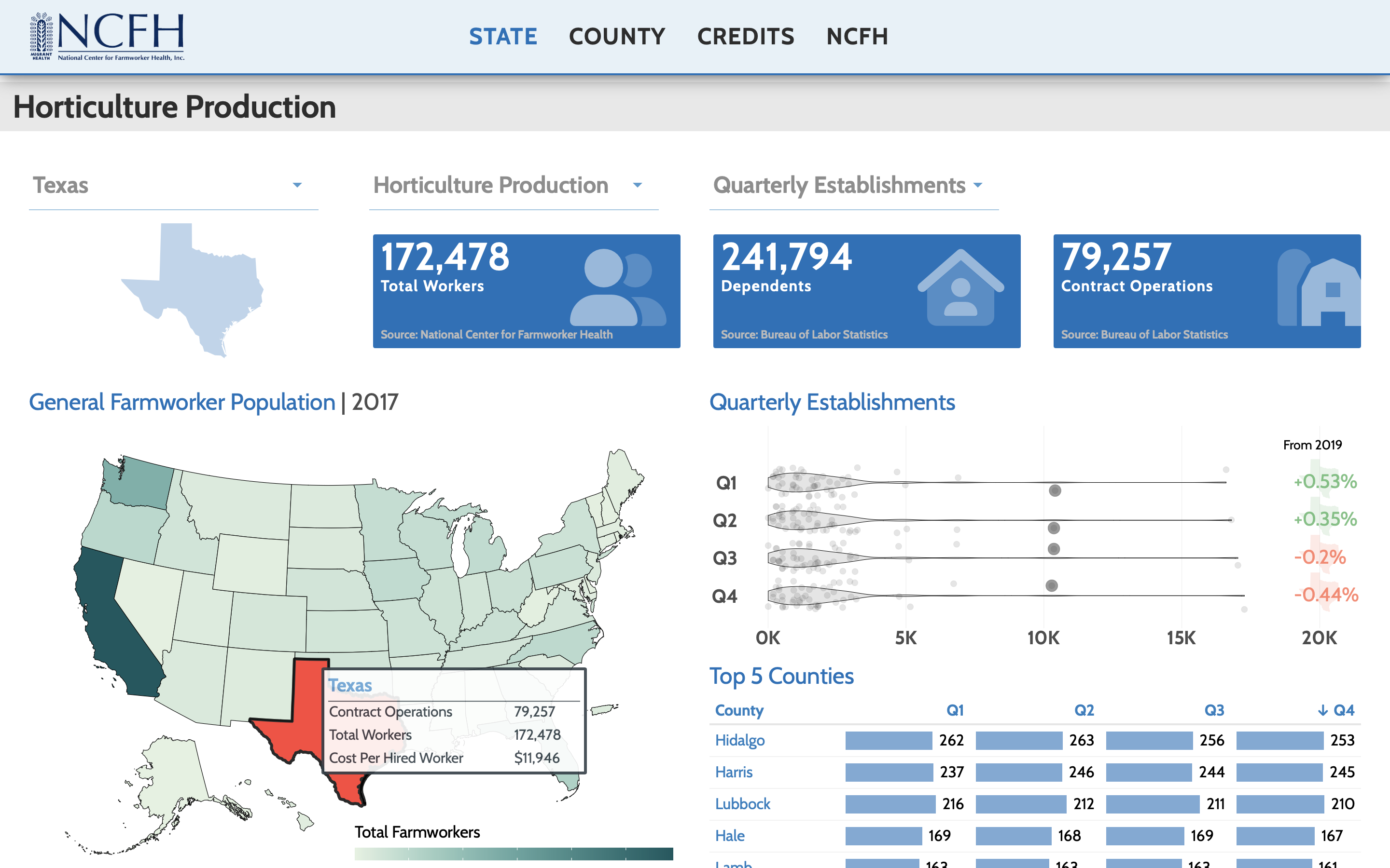 ] --- # Websites: `blogdown` + `distill` .pull-left[ .center[#### [Blogdown](https://pkgs.rstudio.com/blogdown/)]  ] .pull-right[ .center[#### [Distill](https://pkgs.rstudio.com/distill/)]  ] --- # Books: `bookdown` .rmd-img[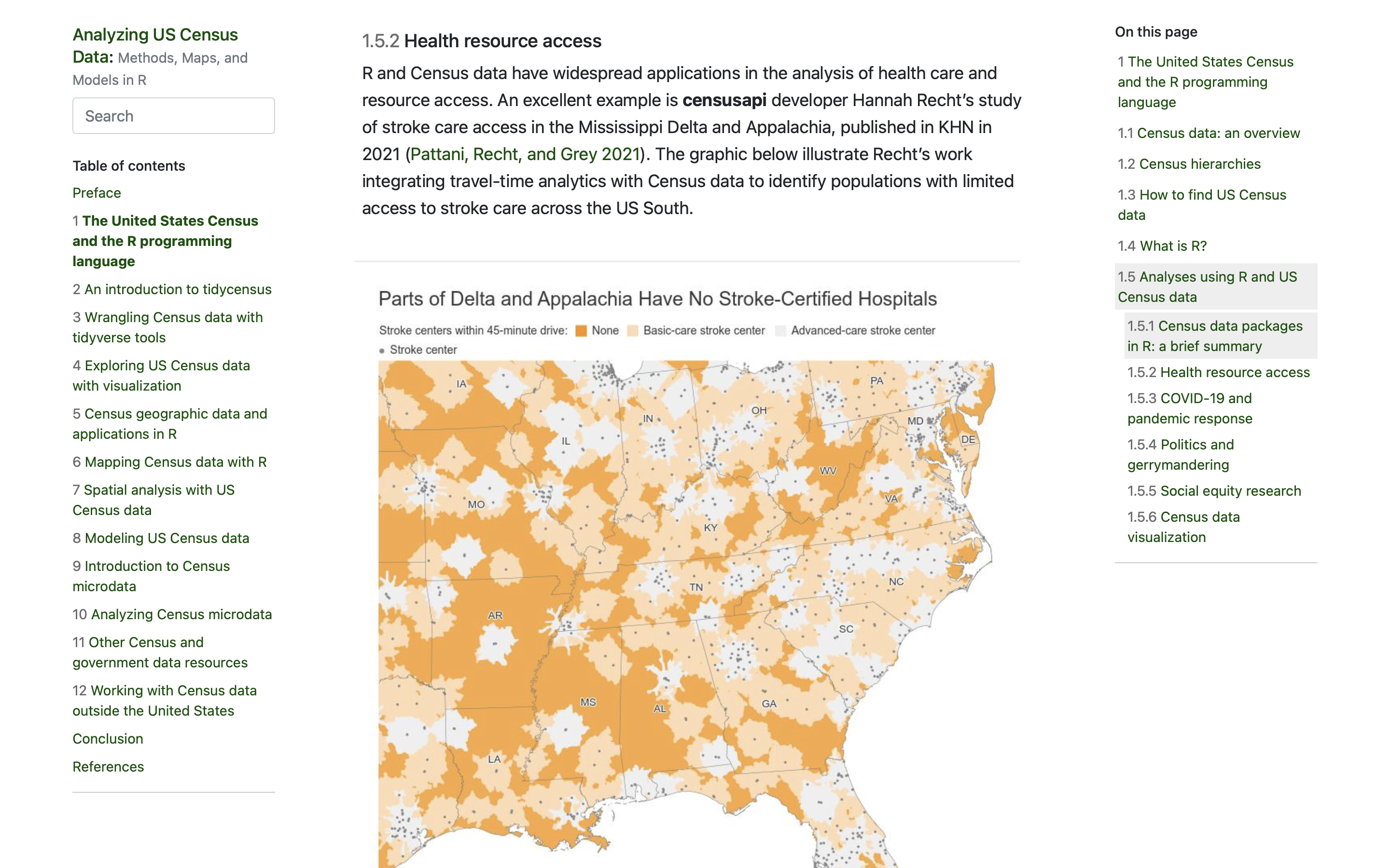] --- # Documents: `rmarkdown` .rmd-img[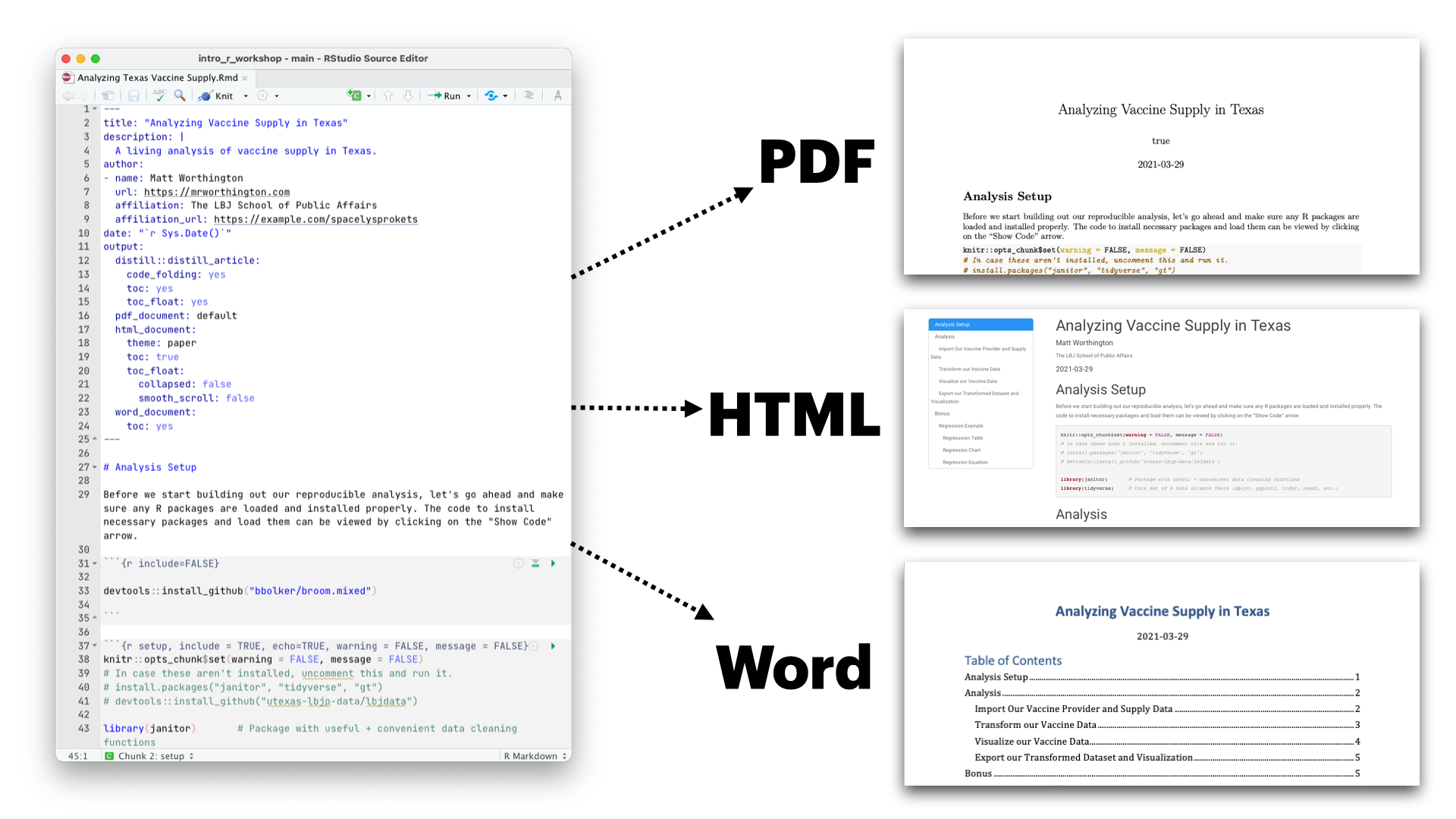] --- # Like anything, this is a journey... .rmd-img[] --- class: journey-bg, section, center, middle, inverse # Let's get started 👟 --- # Downloading Materials .pull-left[ ### Today's Agenda .b--gray.ba.bw2.ma2.shadow-1[ * Navigating Rstudio * Rstudio Interface * R Projects * R Markdown - Markdown Text - Code Chunks * Creating Nice Reports * PDF * Word * HTML * Getting Data You Need * Things People Give You * Things That Live Online * Making Good Charts * Exporting Data & Charts ] ] .pull-right[ ### Today's Materials .b--gray.ba.bw2.ma2.pa2.shadow-1[ #### What You Should Download * [**Rmarkdown Analysis** ](tinyurl.com/TXVaxUptake): tinyurl.com/TXVaxUptake #### What You Should Reference Later * [**Today's Slides**](slides.lbjdata.org/course_workshops/abner/intro_r_workshop/intro_slide) * [**The Published Analysis**](https://demos.lbjdata.org/vaccine_uptake/analyzing-vacine-uptake) ] ] --- background-image: url('assets/images/rstudio_hex.png') background-size: cover class: center, bottom --- # Downloading The Materials * [**Rmarkdown Analysis** ](tinyurl.com/TXVaxUptake): tinyurl.com/TXVaxUptake  --- # Open the `.Rproj` file .rmd-img[] --- background-image: url('https://utexas-lbjp-data.github.io/assets/rmarkdown/slide_17.jpeg') background-size: cover class: center, bottom, inverse --- background-image: url('https://utexas-lbjp-data.github.io/assets/rmarkdown/slide_18.jpeg') background-size: cover class: center, bottom, inverse --- background-image: url('assets/images/tidyverse_hex.png') background-size: cover class: center, bottom, inverse --- background-image: url('assets/images/tidyverse_network.png') background-size: cover class: center, bottom, inverse animated fadeIn --- background-image: url('assets/images/tidyverse_data_lifecycle_map.png') background-size: cover class: center, bottom, inverse animated fadeIn --- background-image: url('assets/images/lifecycle_focus.png') background-size: cover class: center, bottom, inverse animated fadeIn --- background-image: url('assets/images/what_todays_focus_will_be.png') background-size: cover class: center, bottom, inverse animated animate fadeIn --- background-image: url('assets/images/marie_kondo.png') background-size: cover class: center, bottom, inverse animated fadeIn --- # What is R Markdown? .pull-left.b--gray.ba.bw2.ma2.pa4.shadow-1[ * ["An authoring framework for data science."](https://rmarkdown.rstudio.com/lesson-1.html) (✔️) * [A document format (.Rmd)](https://bookdown.org/yihui/rmarkdown/). (✔️) * [An R package named rmarkdown](https://rmarkdown.rstudio.com/docs/). (✔️) * ["A file format for making dynamic documents with R."](https://rmarkdown.rstudio.com/articles_intro.html) (✔️) * ["A tool for integrating text, code, and results."](https://r4ds.had.co.nz/communicate-intro.html) (✔️) * ["A computational document."](http://radar.oreilly.com/2011/07/wolframs-computational-documen.html) (✔️) * Wizardry. (🧙️) ] .pull-right[ .rmd-small[] ] .tl.burntorange[ Courtesy of Alison Presmanes Hill ([@apreshill](https://twitter.com/apreshill)) ] --- background-image: url('https://utexas-lbjp-data.github.io/assets/rmarkdown/slide_15.jpeg') background-size: cover class: center, bottom, inverse --- background-image: url('https://utexas-lbjp-data.github.io/assets/rmarkdown/slide_16.jpeg') background-size: cover class: center, bottom, inverse --- background-image: url('https://utexas-lbjp-data.github.io/assets/rmarkdown/slide_17.jpeg') background-size: cover class: center, bottom, inverse --- background-image: url('https://utexas-lbjp-data.github.io/assets/rmarkdown/slide_18.jpeg') background-size: cover class: center, bottom, inverse --- background-image: url('https://utexas-lbjp-data.github.io/assets/rmarkdown/slide_19.jpeg') background-size: cover class: center, bottom, inverse --- background-image: url('https://utexas-lbjp-data.github.io/assets/rmarkdown/slide_20.jpeg') background-size: cover class: center, bottom, inverse --- background-image: url('https://utexas-lbjp-data.github.io/assets/rmarkdown/slide_21.jpeg') background-size: cover class: center, bottom, inverse --- background-image: url('https://utexas-lbjp-data.github.io/assets/rmarkdown/slide_22.jpeg') background-size: cover class: center, bottom, inverse --- background-image: url('https://utexas-lbjp-data.github.io/assets/rmarkdown/slide_23.jpeg') background-size: cover class: center, bottom, inverse --- background-image: url('https://utexas-lbjp-data.github.io/assets/rmarkdown/slide_24.jpeg') background-size: cover class: center, bottom, inverse --- background-image: url('https://utexas-lbjp-data.github.io/assets/rmarkdown/slide_25.jpeg') background-size: cover class: center, bottom, inverse --- background-image: url('https://utexas-lbjp-data.github.io/assets/rmarkdown/slide_26.jpeg') background-size: cover class: center, bottom, inverse --- background-image: url('https://utexas-lbjp-data.github.io/assets/rmarkdown/slide_27.jpeg') background-size: cover class: center, bottom, inverse --- background-image: url('https://utexas-lbjp-data.github.io/assets/rmarkdown/slide_28.jpeg') background-size: cover class: center, bottom, inverse --- background-image: url('https://utexas-lbjp-data.github.io/assets/rmarkdown/slide_29.jpeg') background-size: cover class: center, bottom, inverse --- background-image: url('https://utexas-lbjp-data.github.io/assets/rmarkdown/slide_30.jpeg') background-size: cover class: center, bottom, inverse --- background-image: url('https://utexas-lbjp-data.github.io/assets/rmarkdown/slide_31.jpeg') background-size: cover class: center, bottom, inverse --- background-image: url('https://utexas-lbjp-data.github.io/assets/rmarkdown/slide_32.jpeg') background-size: cover class: center, bottom, inverse --- background-image: url('https://utexas-lbjp-data.github.io/assets/rmarkdown/slide_33.jpeg') background-size: cover class: center, bottom, inverse --- background-image: url('https://utexas-lbjp-data.github.io/assets/rmarkdown/slide_34.jpeg') background-size: cover class: center, bottom, inverse --- background-image: url('https://utexas-lbjp-data.github.io/assets/rmarkdown/slide_35.jpeg') background-size: cover class: center, bottom, inverse --- background-image: url('https://utexas-lbjp-data.github.io/assets/rmarkdown/slide_36.jpeg') background-size: cover class: center, bottom, inverse --- class: middle .pull-left[ ### Writing in Markdown If you're not familiar with Markdown, that's okay. If you're like me, you grew up using things like Microsoft Office and Google Docs to write, so you're probably not familiar with markdown, but Markdown is a lot easier. So... what is it? Markdown is just an easy way to write formatted text. Like anything else, it takes practice, but is used widely in popular writing apps like [Bear](https://bear.app), [iA Writer](https://ia.net/writer), [Ulysses](https://ulysses.app). For the purposes of this workshop, we'll use it in an RStudio document tool called "[Rmarkdown](https://rmarkdown.rstudio.com)". Here's a quick way to get familiar with writing in Markdown: .bg--burntorange.b--text-color.ba.bw2.br3.shadow-5.ph4.mt5.f7[ *__Note__: If writing in Markdown still feels weird, don't worry. You can also use R Markdown's Visual Markdown Editor.* ] ] .pull-right[  * **First, visit this link:** Go to [https://commonmark.org/help/tutorial/](https://commonmark.org/help/tutorial/) * **Then, do the 10-minute tutorial:** It's a bit of time, but goes quick and will help you have a better grasp on writing in markdown. * **Finally, bookmark this site**: [https://commonmark.org/help/](https://commonmark.org/help/) ] --- background-image: url('https://utexas-lbjp-data.github.io/assets/rmarkdown/slide_38.jpeg') background-size: cover class: center, bottom, inverse --- background-image: url('https://utexas-lbjp-data.github.io/assets/rmarkdown/slide_39.jpeg') background-size: cover class: center, bottom, inverse --- background-image: url('https://utexas-lbjp-data.github.io/assets/rmarkdown/slide_40.jpeg') background-size: cover class: center, bottom, inverse --- background-image: url('https://utexas-lbjp-data.github.io/assets/rmarkdown/slide_41.jpeg') background-size: cover class: center, bottom, inverse --- background-image: url('https://utexas-lbjp-data.github.io/assets/rmarkdown/slide_42.jpeg') background-size: cover class: center, bottom, inverse --- background-image: url('https://utexas-lbjp-data.github.io/assets/rmarkdown/slide_43.jpeg') background-size: cover class: center, bottom, inverse --- background-image: url('https://utexas-lbjp-data.github.io/assets/rmarkdown/slide_44.jpeg') background-size: cover class: center, bottom, inverse --- background-image: url('https://utexas-lbjp-data.github.io/assets/rmarkdown/slide_45.jpeg') background-size: cover class: center, bottom, inverse --- background-image: url('https://utexas-lbjp-data.github.io/assets/rmarkdown/slide_46.jpeg') background-size: cover class: center, bottom, inverse --- background-image: url('https://utexas-lbjp-data.github.io/assets/rmarkdown/slide_47.jpeg') background-size: cover class: center, bottom, inverse --- class: title center pipe-page # `|>` and `%>%` <code class ='r hljs remark-code'><b>leave_house</b>(<b>get_dressed</b>(<b>get_out_of_bed</b>(<b>wake_up</b>(<span style='color:#bf5700'>me</span>, <span style='color:#005f86'>time</span> = <span style='color:#bf5700'>"8:00"</span>), <span style='color:#005f86'>side</span> = <span style='color:#bf5700'>"correct"</span>), <span style='color:#005f86'>pants</span> = <span style='color:#bf5700'>TRUE</span>, <span style='color:#005f86'>shirt</span> = <span style='color:#bf5700'>TRUE</span>), <span style='color:#005f86'>car</span> = <span style='color:#bf5700'>TRUE</span>, <span style='color:#005f86'>bike</span> = <span style='color:#bf5700'>FALSE</span>)</code> -- <code class ='r hljs remark-code'>me <span style='background-color:#ffff7f'>|></span> <br> <b>wake_up</b>(<span style='color:#005f86'>time</span> = <span style='color:#bf5700'>"8:00"</span>) <span style='background-color:#ffff7f'>|></span> <br> <b>get_out_of_bed</b>(<span style='color:#005f86'>side</span> = <span style='color:#bf5700'>"correct"</span>) <span style='background-color:#ffff7f'>|></span> <br> <b>get_dressed</b>(<span style='color:#005f86'>pants</span> = <span style='color:#bf5700'>TRUE</span>, <span style='color:#005f86'>shirt</span> = <span style='color:#bf5700'>TRUE</span>) <span style='background-color:#ffff7f'>|></span> <br> <b>leave_house</b>(<span style='color:#005f86'>car</span> = <span style='color:#bf5700'>TRUE</span>, <span style='color:#005f86'>bike</span> = <span style='color:#bf5700'>FALSE</span>)</code> .tl.footnote-small[ Courtesy of Andrew Heiss ([@andrewheiss](https://twitter.com/andrewheiss)) ] --- class: vaccine-bg, section, center, middle, inverse # And Now... The Analysis --- # Package Setup Under the **Analysis Setup** section, there's a chunk tagged `setup` that starts on line 32. ```r knitr::opts_chunk$set(warning = FALSE, message = FALSE) # In case these aren't installed already from the prework, uncomment the next three lines and run them. # install.packages(c("rmarkdown", "tidyverse", "tidycensus", "distill", "devtools")) # install.packages(c("janitor", "readxl")) # devtools::install_github("utexas-lbjp-data/lbjdata") library(janitor) # Package with useful + convenient data cleaning functions library(readxl) # Package with useful functions for working with Excel Files library(tidyverse) # Core Set of R Data Science Tools (dplyr, ggplot2, tidyr, readr, etc.) library(lbjdata) # LBJ Data Package which has the ggplot2 themes ``` -- ### What's happening here? .b--burntorange.ba.bw2.ma2.pa2.shadow-1[ Whenever you see `library(...)`, it means we are loading the packages into our Rmarkdown document so we can use the functions inside of them? In other words, we're pulling out the spellbooks and getting ready to do some data magic. ] --- ## `janitor::clean_names()` **What it does:** Makes all column names machine readble (huge time saver): .rmd-small[] .tl.burntorange[ Credit: ([@allison_horst](https://twitter.com/allison_horst)) ] --- # Importing Our Data .pull-left[ **Step 1: Downloading Our Data** ```r vax_url <- "https://dshs.texas.gov/immunize/covid19/COVID-19-Vaccine-Data-by-County.xls" download.file(url=vax_url, destfile = "raw_data/tx_vaccine_uptake.xlsx") ``` **Step 2: Import the Downloaded Data** ```r vaccine_data_raw <- readxl::read_excel(path = "raw_data/tx_vaccine_uptake.xlsx", sheet = "By County") |> janitor::clean_names() # This function makes column headers machine readable dplyr::glimpse(vaccine_data_raw) # glimpse() lets you preview a data object ``` ] .pull-right[ .rmd-img[] ] --- count: false # Importing - step by step view .panel1-import-data-real-auto[ ```r *readxl::read_excel(path = "raw_data/tx_vaccine_uptake.xlsx", * sheet = "By County") ``` ] .panel2-import-data-real-auto[ ``` # A tibble: 259 × 13 `County Name` `Public Health Reg… `Total Doses All… `Vaccine Doses Ad… <chr> <chr> <dbl> <chr> 1 Texas -- 27513735 29823734 2 Federal Long-Term C… -- 720525 -- 3 Federal Pharmacy Re… -- 5509700 -- 4 Anderson 4/5N 17870 39858 5 Andrews 9/10 6100 14186 6 Angelina 4/5N 58100 66563 7 Aransas 11 6840 25549 8 Archer 2/3 3200 7005 9 Armstrong 1 2100 1272 10 Atascosa 8 19000 43015 # … with 249 more rows, and 9 more variables: # People Vaccinated with at least One Dose <chr>, # People Fully Vaccinated <chr>, Population 12+ <chr>, Population, 16+ <chr>, # Population, 65+ <chr>, Population, Phase 1A Healthcare Workers <chr>, # Population, Phase 1A Long-term Care Residents <chr>, # Population, 16-64 Any Medical Condition <chr>, # Population, Education and Child Care Personnel <chr> ``` ] --- count: false # Importing - step by step view .panel1-import-data-real-auto[ ```r readxl::read_excel(path = "raw_data/tx_vaccine_uptake.xlsx", sheet = "By County") %>% * janitor::clean_names() ``` ] .panel2-import-data-real-auto[ ``` # A tibble: 259 × 13 county_name public_health_regi… total_doses_allo… vaccine_doses_adm… <chr> <chr> <dbl> <chr> 1 Texas -- 27513735 29823734 2 Federal Long-Term C… -- 720525 -- 3 Federal Pharmacy Re… -- 5509700 -- 4 Anderson 4/5N 17870 39858 5 Andrews 9/10 6100 14186 6 Angelina 4/5N 58100 66563 7 Aransas 11 6840 25549 8 Archer 2/3 3200 7005 9 Armstrong 1 2100 1272 10 Atascosa 8 19000 43015 # … with 249 more rows, and 9 more variables: # people_vaccinated_with_at_least_one_dose <chr>, # people_fully_vaccinated <chr>, population_12 <chr>, population_16 <chr>, # population_65 <chr>, population_phase_1a_healthcare_workers <chr>, # population_phase_1a_long_term_care_residents <chr>, # population_16_64_any_medical_condition <chr>, # population_education_and_child_care_personnel <chr> ``` ] --- count: false # Importing - step by step view .panel1-import-data-real-auto[ ```r readxl::read_excel(path = "raw_data/tx_vaccine_uptake.xlsx", sheet = "By County") %>% janitor::clean_names() ``` ] .panel2-import-data-real-auto[ ``` # A tibble: 259 × 13 county_name public_health_regi… total_doses_allo… vaccine_doses_adm… <chr> <chr> <dbl> <chr> 1 Texas -- 27513735 29823734 2 Federal Long-Term C… -- 720525 -- 3 Federal Pharmacy Re… -- 5509700 -- 4 Anderson 4/5N 17870 39858 5 Andrews 9/10 6100 14186 6 Angelina 4/5N 58100 66563 7 Aransas 11 6840 25549 8 Archer 2/3 3200 7005 9 Armstrong 1 2100 1272 10 Atascosa 8 19000 43015 # … with 249 more rows, and 9 more variables: # people_vaccinated_with_at_least_one_dose <chr>, # people_fully_vaccinated <chr>, population_12 <chr>, population_16 <chr>, # population_65 <chr>, population_phase_1a_healthcare_workers <chr>, # population_phase_1a_long_term_care_residents <chr>, # population_16_64_any_medical_condition <chr>, # population_education_and_child_care_personnel <chr> ``` ] <style> .panel1-import-data-real-auto { color: black; width: 38.6060606060606%; hight: 32%; float: left; padding-left: 1%; font-size: 80% } .panel2-import-data-real-auto { color: black; width: 59.3939393939394%; hight: 32%; float: left; padding-left: 1%; font-size: 80% } .panel3-import-data-real-auto { color: black; width: NA%; hight: 33%; float: left; padding-left: 1%; font-size: 80% } </style> --- ## `dplyr::select()` **What it does:** Selects your preferred columns from your data set. <iframe width="750" height = "416" src="https://video.twimg.com/tweet_video/E-D3IWxWYAEIk51.mp4" frameborder="0" style = "border: solid 0px #ffffff" color = "white" modestbranding = "1" allow="accelerometer; autoplay; clipboard-write; encrypted-media; gyroscope; picture-in-picture" allowfullscreen data-external="1"></iframe> .tl.burntorange[ Credit: ([@illustratedbyte](https://twitter.com/illustratedbyte)) ] --- ## `dplyr::mutate()` **What it does:** Creates or transforms a variable (column) while keeping the existing ones: .rmd-tiny[] .tl.burntorange[ Credit: ([@allison_horst](https://twitter.com/allison_horst)) ] --- ## `dplyr::filter()` **What it does:** Subsets rows based on your conditions .rmd-small[] .tl.burntorange[ Credit: ([@allison_horst](https://twitter.com/allison_horst)) ] --- # Working With Our Data ### Step 1 ```r vaccine_uptake <- vaccine_data_raw %>% select(county_name, people_fully_vaccinated, population_12) %>% # Pull the three columns we need mutate(people_fully_vaccinated = as.numeric(people_fully_vaccinated), # Reclassify Character Data As Numeric population_12 = as.numeric(population_12)) %>% mutate(pct_uptake = round(people_fully_vaccinated/population_12, digits = 4)) %>% # Create PCT Column filter(county_name!="Texas", # Filter out 'Texas' value county_name!="Other", # Filter our 'Other' value county_name!="Federal Long-Term Care Vaccination Program", # Filter our Federal Programs county_name!="Federal Pharmacy Retail Vaccination Program") ``` ``` # A tibble: 254 × 4 county_name people_fully_vaccinated population_12 pct_uptake <chr> <dbl> <dbl> <dbl> 1 Anderson 19254 50661 0.380 2 Andrews 6589 14863 0.443 3 Angelina 31593 72486 0.436 4 Aransas 12099 20834 0.581 5 Archer 3459 7388 0.468 6 Armstrong 597 1584 0.377 7 Atascosa 20178 41738 0.483 8 Austin 12388 25335 0.489 9 Bailey 2274 5603 0.406 10 Bandera 8709 20596 0.423 # … with 244 more rows ``` --- count: false # Working with Data - Step 1 .panel1-create-pct-column-real-auto[ ```r *vaccine_data_raw ``` ] .panel2-create-pct-column-real-auto[ ``` # A tibble: 259 × 13 county_name public_health_regi… total_doses_allo… vaccine_doses_adm… <chr> <chr> <dbl> <chr> 1 Texas -- 27513735 29823734 2 Federal Long-Term C… -- 720525 -- 3 Federal Pharmacy Re… -- 5509700 -- 4 Anderson 4/5N 17870 39858 5 Andrews 9/10 6100 14186 6 Angelina 4/5N 58100 66563 7 Aransas 11 6840 25549 8 Archer 2/3 3200 7005 9 Armstrong 1 2100 1272 10 Atascosa 8 19000 43015 # … with 249 more rows, and 9 more variables: # people_vaccinated_with_at_least_one_dose <chr>, # people_fully_vaccinated <chr>, population_12 <chr>, population_16 <chr>, # population_65 <chr>, population_phase_1a_healthcare_workers <chr>, # population_phase_1a_long_term_care_residents <chr>, # population_16_64_any_medical_condition <chr>, # population_education_and_child_care_personnel <chr> ``` ] --- count: false # Working with Data - Step 1 .panel1-create-pct-column-real-auto[ ```r vaccine_data_raw %>% * select(county_name, people_fully_vaccinated, population_12) # Pull the three columns we need ``` ] .panel2-create-pct-column-real-auto[ ``` # A tibble: 259 × 3 county_name people_fully_vacci… population_12 <chr> <chr> <chr> 1 Texas 14183523 24068624 2 Federal Long-Term Care Vaccination Program -- -- 3 Federal Pharmacy Retail Vaccination Program -- -- 4 Anderson 19254 50661 5 Andrews 6589 14863 6 Angelina 31593 72486 7 Aransas 12099 20834 8 Archer 3459 7388 9 Armstrong 597 1584 10 Atascosa 20178 41738 # … with 249 more rows ``` ] --- count: false # Working with Data - Step 1 .panel1-create-pct-column-real-auto[ ```r vaccine_data_raw %>% select(county_name, people_fully_vaccinated, population_12) %>% # Pull the three columns we need * mutate(people_fully_vaccinated = as.numeric(people_fully_vaccinated), # Reclassify Character Data As Numeric * population_12 = as.numeric(population_12)) ``` ] .panel2-create-pct-column-real-auto[ ``` # A tibble: 259 × 3 county_name people_fully_vacci… population_12 <chr> <dbl> <dbl> 1 Texas 14183523 24068624 2 Federal Long-Term Care Vaccination Program NA NA 3 Federal Pharmacy Retail Vaccination Program NA NA 4 Anderson 19254 50661 5 Andrews 6589 14863 6 Angelina 31593 72486 7 Aransas 12099 20834 8 Archer 3459 7388 9 Armstrong 597 1584 10 Atascosa 20178 41738 # … with 249 more rows ``` ] --- count: false # Working with Data - Step 1 .panel1-create-pct-column-real-auto[ ```r vaccine_data_raw %>% select(county_name, people_fully_vaccinated, population_12) %>% # Pull the three columns we need mutate(people_fully_vaccinated = as.numeric(people_fully_vaccinated), # Reclassify Character Data As Numeric population_12 = as.numeric(population_12)) %>% * mutate(pct_uptake = round(people_fully_vaccinated/population_12, digits = 4)) # Create PCT Column ``` ] .panel2-create-pct-column-real-auto[ ``` # A tibble: 259 × 4 county_name people_fully_vaccin… population_12 pct_uptake <chr> <dbl> <dbl> <dbl> 1 Texas 14183523 24068624 0.589 2 Federal Long-Term Care Vaccina… NA NA NA 3 Federal Pharmacy Retail Vaccin… NA NA NA 4 Anderson 19254 50661 0.380 5 Andrews 6589 14863 0.443 6 Angelina 31593 72486 0.436 7 Aransas 12099 20834 0.581 8 Archer 3459 7388 0.468 9 Armstrong 597 1584 0.377 10 Atascosa 20178 41738 0.483 # … with 249 more rows ``` ] --- count: false # Working with Data - Step 1 .panel1-create-pct-column-real-auto[ ```r vaccine_data_raw %>% select(county_name, people_fully_vaccinated, population_12) %>% # Pull the three columns we need mutate(people_fully_vaccinated = as.numeric(people_fully_vaccinated), # Reclassify Character Data As Numeric population_12 = as.numeric(population_12)) %>% mutate(pct_uptake = round(people_fully_vaccinated/population_12, digits = 4)) %>% # Create PCT Column * filter(county_name!="Texas", # Filter out 'Texas' value * county_name!="Other", # Filter our 'Other' value * county_name!="Federal Long-Term Care Vaccination Program", # Filter our Federal Programs * county_name!="Federal Pharmacy Retail Vaccination Program") ``` ] .panel2-create-pct-column-real-auto[ ``` # A tibble: 254 × 4 county_name people_fully_vaccinated population_12 pct_uptake <chr> <dbl> <dbl> <dbl> 1 Anderson 19254 50661 0.380 2 Andrews 6589 14863 0.443 3 Angelina 31593 72486 0.436 4 Aransas 12099 20834 0.581 5 Archer 3459 7388 0.468 6 Armstrong 597 1584 0.377 7 Atascosa 20178 41738 0.483 8 Austin 12388 25335 0.489 9 Bailey 2274 5603 0.406 10 Bandera 8709 20596 0.423 # … with 244 more rows ``` ] <style> .panel1-create-pct-column-real-auto { color: black; width: 38.6060606060606%; hight: 32%; float: left; padding-left: 1%; font-size: 80% } .panel2-create-pct-column-real-auto { color: black; width: 59.3939393939394%; hight: 32%; float: left; padding-left: 1%; font-size: 80% } .panel3-create-pct-column-real-auto { color: black; width: NA%; hight: 33%; float: left; padding-left: 1%; font-size: 80% } </style> --- # Working With Our Data ### Step 2 ```r ranked_uptake <- vaccine_uptake %>% # Create New Object mutate(uptake_rank = dense_rank(desc(pct_uptake))) %>% # Create Rank Column filter(uptake_rank <= 10) %>% # Filter only for Top 10 counties arrange(uptake_rank) # Sort by rank ``` ``` # A tibble: 10 × 5 county_name people_fully_vaccinated population_12 pct_uptake uptake_rank <chr> <dbl> <dbl> <dbl> <int> 1 Presidio 5182 5392 0.961 1 2 Webb 182570 215919 0.846 2 3 Starr 41696 49864 0.836 3 4 Cameron 260316 339698 0.766 4 5 Maverick 35051 46417 0.755 5 6 Hidalgo 511412 681678 0.750 6 7 El Paso 512785 688420 0.745 7 8 Fort Bend 484674 665167 0.729 8 9 Travis 750079 1092827 0.686 9 10 Hudspeth 2822 4139 0.682 10 ``` --- count: false # Working with Data - Step 2 .panel1-rank-and-limit-real-auto[ ```r *vaccine_uptake # Create New Object ``` ] .panel2-rank-and-limit-real-auto[ ``` # A tibble: 254 × 4 county_name people_fully_vaccinated population_12 pct_uptake <chr> <dbl> <dbl> <dbl> 1 Anderson 19254 50661 0.380 2 Andrews 6589 14863 0.443 3 Angelina 31593 72486 0.436 4 Aransas 12099 20834 0.581 5 Archer 3459 7388 0.468 6 Armstrong 597 1584 0.377 7 Atascosa 20178 41738 0.483 8 Austin 12388 25335 0.489 9 Bailey 2274 5603 0.406 10 Bandera 8709 20596 0.423 # … with 244 more rows ``` ] --- count: false # Working with Data - Step 2 .panel1-rank-and-limit-real-auto[ ```r vaccine_uptake %>% # Create New Object * mutate(uptake_rank = dense_rank(desc(pct_uptake))) # Create Rank Column ``` ] .panel2-rank-and-limit-real-auto[ ``` # A tibble: 254 × 5 county_name people_fully_vaccinated population_12 pct_uptake uptake_rank <chr> <dbl> <dbl> <dbl> <int> 1 Anderson 19254 50661 0.380 181 2 Andrews 6589 14863 0.443 99 3 Angelina 31593 72486 0.436 109 4 Aransas 12099 20834 0.581 32 5 Archer 3459 7388 0.468 79 6 Armstrong 597 1584 0.377 187 7 Atascosa 20178 41738 0.483 68 8 Austin 12388 25335 0.489 65 9 Bailey 2274 5603 0.406 147 10 Bandera 8709 20596 0.423 127 # … with 244 more rows ``` ] --- count: false # Working with Data - Step 2 .panel1-rank-and-limit-real-auto[ ```r vaccine_uptake %>% # Create New Object mutate(uptake_rank = dense_rank(desc(pct_uptake))) %>% # Create Rank Column * filter(uptake_rank <= 10) # Filter only for Top 10 counties ``` ] .panel2-rank-and-limit-real-auto[ ``` # A tibble: 10 × 5 county_name people_fully_vaccinated population_12 pct_uptake uptake_rank <chr> <dbl> <dbl> <dbl> <int> 1 Cameron 260316 339698 0.766 4 2 El Paso 512785 688420 0.745 7 3 Fort Bend 484674 665167 0.729 8 4 Hidalgo 511412 681678 0.750 6 5 Hudspeth 2822 4139 0.682 10 6 Maverick 35051 46417 0.755 5 7 Presidio 5182 5392 0.961 1 8 Starr 41696 49864 0.836 3 9 Travis 750079 1092827 0.686 9 10 Webb 182570 215919 0.846 2 ``` ] --- count: false # Working with Data - Step 2 .panel1-rank-and-limit-real-auto[ ```r vaccine_uptake %>% # Create New Object mutate(uptake_rank = dense_rank(desc(pct_uptake))) %>% # Create Rank Column filter(uptake_rank <= 10) %>% # Filter only for Top 10 counties * arrange(uptake_rank) # Sort by rank ``` ] .panel2-rank-and-limit-real-auto[ ``` # A tibble: 10 × 5 county_name people_fully_vaccinated population_12 pct_uptake uptake_rank <chr> <dbl> <dbl> <dbl> <int> 1 Presidio 5182 5392 0.961 1 2 Webb 182570 215919 0.846 2 3 Starr 41696 49864 0.836 3 4 Cameron 260316 339698 0.766 4 5 Maverick 35051 46417 0.755 5 6 Hidalgo 511412 681678 0.750 6 7 El Paso 512785 688420 0.745 7 8 Fort Bend 484674 665167 0.729 8 9 Travis 750079 1092827 0.686 9 10 Hudspeth 2822 4139 0.682 10 ``` ] --- count: false # Working with Data - Step 2 .panel1-rank-and-limit-real-auto[ ```r vaccine_uptake %>% # Create New Object mutate(uptake_rank = dense_rank(desc(pct_uptake))) %>% # Create Rank Column filter(uptake_rank <= 10) %>% # Filter only for Top 10 counties arrange(uptake_rank) # Sort by rank ``` ] .panel2-rank-and-limit-real-auto[ ``` # A tibble: 10 × 5 county_name people_fully_vaccinated population_12 pct_uptake uptake_rank <chr> <dbl> <dbl> <dbl> <int> 1 Presidio 5182 5392 0.961 1 2 Webb 182570 215919 0.846 2 3 Starr 41696 49864 0.836 3 4 Cameron 260316 339698 0.766 4 5 Maverick 35051 46417 0.755 5 6 Hidalgo 511412 681678 0.750 6 7 El Paso 512785 688420 0.745 7 8 Fort Bend 484674 665167 0.729 8 9 Travis 750079 1092827 0.686 9 10 Hudspeth 2822 4139 0.682 10 ``` ] <style> .panel1-rank-and-limit-real-auto { color: black; width: 38.6060606060606%; hight: 32%; float: left; padding-left: 1%; font-size: 80% } .panel2-rank-and-limit-real-auto { color: black; width: 59.3939393939394%; hight: 32%; float: left; padding-left: 1%; font-size: 80% } .panel3-rank-and-limit-real-auto { color: black; width: NA%; hight: 33%; float: left; padding-left: 1%; font-size: 80% } </style> --- # The Basics of a ggplot2 chart .pull-left[ ```r library(ggplot2) library(ggthemes) diamonds |> # Call On Your Dataset ggplot() + # Draw A Canvas aes(cut, fill = cut) + # Define How The Data Gets Mapped geom_bar(show.legend = FALSE) + # Define What Kind of Chart to Draw labs( x = "Cut", # Specify X-Axis Label y = "Count", # Specify Y-Axis Label title = "A Fancy diamonds Plot", # Specify Title Label subtitle = "A compelling subtitle", # Specify Subtitle Label caption = "Source: ggplot2 package | Data: 'diamonds'" # Specify Source/Caption Label ) + theme_lbj() + # Add The LBJ Theme theme(plot.title = element_text(color = "#bf5700")) + # Modify Title's Color ggthemes::scale_fill_tableau(palette = "Color Blind") # Add A Color Blind Friendly Palette ``` ] .pull-right[ <img src="intro_slides_files/figure-html/fancy_diamonds-1.png" width="504" /> ] --- count: false # A step by step view .panel1-fancy_diamonds-auto[ ```r *library(ggplot2) ``` ] .panel2-fancy_diamonds-auto[ ] --- count: false # A step by step view .panel1-fancy_diamonds-auto[ ```r library(ggplot2) *library(ggthemes) ``` ] .panel2-fancy_diamonds-auto[ ] --- count: false # A step by step view .panel1-fancy_diamonds-auto[ ```r library(ggplot2) library(ggthemes) *diamonds # Call On Your Dataset ``` ] .panel2-fancy_diamonds-auto[ ``` # A tibble: 53,940 × 10 carat cut color clarity depth table price x y z <dbl> <ord> <ord> <ord> <dbl> <dbl> <int> <dbl> <dbl> <dbl> 1 0.23 Ideal E SI2 61.5 55 326 3.95 3.98 2.43 2 0.21 Premium E SI1 59.8 61 326 3.89 3.84 2.31 3 0.23 Good E VS1 56.9 65 327 4.05 4.07 2.31 4 0.29 Premium I VS2 62.4 58 334 4.2 4.23 2.63 5 0.31 Good J SI2 63.3 58 335 4.34 4.35 2.75 6 0.24 Very Good J VVS2 62.8 57 336 3.94 3.96 2.48 7 0.24 Very Good I VVS1 62.3 57 336 3.95 3.98 2.47 8 0.26 Very Good H SI1 61.9 55 337 4.07 4.11 2.53 9 0.22 Fair E VS2 65.1 61 337 3.87 3.78 2.49 10 0.23 Very Good H VS1 59.4 61 338 4 4.05 2.39 # … with 53,930 more rows ``` ] --- count: false # A step by step view .panel1-fancy_diamonds-auto[ ```r library(ggplot2) library(ggthemes) diamonds %>% # Call On Your Dataset * ggplot() # Draw A Canvas ``` ] .panel2-fancy_diamonds-auto[ <img src="intro_slides_files/figure-html/fancy_diamonds_auto_04_output-1.png" width="504" /> ] --- count: false # A step by step view .panel1-fancy_diamonds-auto[ ```r library(ggplot2) library(ggthemes) diamonds %>% # Call On Your Dataset ggplot() + # Draw A Canvas * aes(cut, fill = cut) # Define How The Data Gets Mapped ``` ] .panel2-fancy_diamonds-auto[ <img src="intro_slides_files/figure-html/fancy_diamonds_auto_05_output-1.png" width="504" /> ] --- count: false # A step by step view .panel1-fancy_diamonds-auto[ ```r library(ggplot2) library(ggthemes) diamonds %>% # Call On Your Dataset ggplot() + # Draw A Canvas aes(cut, fill = cut) + # Define How The Data Gets Mapped * geom_bar(show.legend = FALSE) # Define What Kind of Chart to Draw ``` ] .panel2-fancy_diamonds-auto[ <img src="intro_slides_files/figure-html/fancy_diamonds_auto_06_output-1.png" width="504" /> ] --- count: false # A step by step view .panel1-fancy_diamonds-auto[ ```r library(ggplot2) library(ggthemes) diamonds %>% # Call On Your Dataset ggplot() + # Draw A Canvas aes(cut, fill = cut) + # Define How The Data Gets Mapped geom_bar(show.legend = FALSE) + # Define What Kind of Chart to Draw * labs( * x = "Cut", # Specify X-Axis Label * y = "Count", # Specify Y-Axis Label * title = "A Fancy diamonds Plot", # Specify Title Label * subtitle = "A compelling subtitle", # Specify Subtitle Label * caption = "Source: ggplot2 package | Data: 'diamonds'" # Specify Source/Caption Label * ) ``` ] .panel2-fancy_diamonds-auto[ <img src="intro_slides_files/figure-html/fancy_diamonds_auto_07_output-1.png" width="504" /> ] --- count: false # A step by step view .panel1-fancy_diamonds-auto[ ```r library(ggplot2) library(ggthemes) diamonds %>% # Call On Your Dataset ggplot() + # Draw A Canvas aes(cut, fill = cut) + # Define How The Data Gets Mapped geom_bar(show.legend = FALSE) + # Define What Kind of Chart to Draw labs( x = "Cut", # Specify X-Axis Label y = "Count", # Specify Y-Axis Label title = "A Fancy diamonds Plot", # Specify Title Label subtitle = "A compelling subtitle", # Specify Subtitle Label caption = "Source: ggplot2 package | Data: 'diamonds'" # Specify Source/Caption Label ) + * theme_lbj() # Add The LBJ Theme ``` ] .panel2-fancy_diamonds-auto[ <img src="intro_slides_files/figure-html/fancy_diamonds_auto_08_output-1.png" width="504" /> ] --- count: false # A step by step view .panel1-fancy_diamonds-auto[ ```r library(ggplot2) library(ggthemes) diamonds %>% # Call On Your Dataset ggplot() + # Draw A Canvas aes(cut, fill = cut) + # Define How The Data Gets Mapped geom_bar(show.legend = FALSE) + # Define What Kind of Chart to Draw labs( x = "Cut", # Specify X-Axis Label y = "Count", # Specify Y-Axis Label title = "A Fancy diamonds Plot", # Specify Title Label subtitle = "A compelling subtitle", # Specify Subtitle Label caption = "Source: ggplot2 package | Data: 'diamonds'" # Specify Source/Caption Label ) + theme_lbj() + # Add The LBJ Theme * theme(plot.title = element_text(color = "#bf5700")) # Modify Title's Color ``` ] .panel2-fancy_diamonds-auto[ <img src="intro_slides_files/figure-html/fancy_diamonds_auto_09_output-1.png" width="504" /> ] --- count: false # A step by step view .panel1-fancy_diamonds-auto[ ```r library(ggplot2) library(ggthemes) diamonds %>% # Call On Your Dataset ggplot() + # Draw A Canvas aes(cut, fill = cut) + # Define How The Data Gets Mapped geom_bar(show.legend = FALSE) + # Define What Kind of Chart to Draw labs( x = "Cut", # Specify X-Axis Label y = "Count", # Specify Y-Axis Label title = "A Fancy diamonds Plot", # Specify Title Label subtitle = "A compelling subtitle", # Specify Subtitle Label caption = "Source: ggplot2 package | Data: 'diamonds'" # Specify Source/Caption Label ) + theme_lbj() + # Add The LBJ Theme theme(plot.title = element_text(color = "#bf5700")) + # Modify Title's Color * scale_fill_tableau(palette = "Color Blind") # Add A Color Blind Friendly Palette ``` ] .panel2-fancy_diamonds-auto[ <img src="intro_slides_files/figure-html/fancy_diamonds_auto_10_output-1.png" width="504" /> ] --- count: false # A step by step view .panel1-fancy_diamonds-auto[ ```r library(ggplot2) library(ggthemes) diamonds %>% # Call On Your Dataset ggplot() + # Draw A Canvas aes(cut, fill = cut) + # Define How The Data Gets Mapped geom_bar(show.legend = FALSE) + # Define What Kind of Chart to Draw labs( x = "Cut", # Specify X-Axis Label y = "Count", # Specify Y-Axis Label title = "A Fancy diamonds Plot", # Specify Title Label subtitle = "A compelling subtitle", # Specify Subtitle Label caption = "Source: ggplot2 package | Data: 'diamonds'" # Specify Source/Caption Label ) + theme_lbj() + # Add The LBJ Theme theme(plot.title = element_text(color = "#bf5700")) + # Modify Title's Color scale_fill_tableau(palette = "Color Blind") # Add A Color Blind Friendly Palette ``` ] .panel2-fancy_diamonds-auto[ <img src="intro_slides_files/figure-html/fancy_diamonds_auto_11_output-1.png" width="504" /> ] <style> .panel1-fancy_diamonds-auto { color: black; width: 38.6060606060606%; hight: 32%; float: left; padding-left: 1%; font-size: 80% } .panel2-fancy_diamonds-auto { color: black; width: 59.3939393939394%; hight: 32%; float: left; padding-left: 1%; font-size: 80% } .panel3-fancy_diamonds-auto { color: black; width: NA%; hight: 33%; float: left; padding-left: 1%; font-size: 80% } </style> --- # Visualizing Our Data .pull-left[ ```r uptake_chart <- ggplot(ranked_uptake) + aes(x=county_name, y = pct_uptake, fill=pct_uptake) + geom_col() + labs(title = "Leaders of the Vax", subtitle = "Top 10 Counties in Texas for Vaccine Uptake", x = "Vaccine Uptake (%)", y = "County") + lbjdata::theme_lbj(base_size = 10) ``` ] .pull-right[ <img src="intro_slides_files/figure-html/draw-viz-real-1.png" width="504" /> ] --- count: false # Visualizing our Data .panel1-draw-viz-real-auto[ ```r *ggplot(ranked_uptake) ``` ] .panel2-draw-viz-real-auto[ <img src="intro_slides_files/figure-html/draw-viz-real_auto_01_output-1.png" width="504" /> ] --- count: false # Visualizing our Data .panel1-draw-viz-real-auto[ ```r ggplot(ranked_uptake) + * aes(x=county_name, y = pct_uptake, fill=pct_uptake) ``` ] .panel2-draw-viz-real-auto[ <img src="intro_slides_files/figure-html/draw-viz-real_auto_02_output-1.png" width="504" /> ] --- count: false # Visualizing our Data .panel1-draw-viz-real-auto[ ```r ggplot(ranked_uptake) + aes(x=county_name, y = pct_uptake, fill=pct_uptake) + * geom_col() ``` ] .panel2-draw-viz-real-auto[ <img src="intro_slides_files/figure-html/draw-viz-real_auto_03_output-1.png" width="504" /> ] --- count: false # Visualizing our Data .panel1-draw-viz-real-auto[ ```r ggplot(ranked_uptake) + aes(x=county_name, y = pct_uptake, fill=pct_uptake) + geom_col() + * labs(title = "Leaders of the Vax", * subtitle = "Top 10 Counties in Texas for Vaccine Uptake", * x = "Vaccine Uptake (%)", * y = "County") ``` ] .panel2-draw-viz-real-auto[ <img src="intro_slides_files/figure-html/draw-viz-real_auto_04_output-1.png" width="504" /> ] --- count: false # Visualizing our Data .panel1-draw-viz-real-auto[ ```r ggplot(ranked_uptake) + aes(x=county_name, y = pct_uptake, fill=pct_uptake) + geom_col() + labs(title = "Leaders of the Vax", subtitle = "Top 10 Counties in Texas for Vaccine Uptake", x = "Vaccine Uptake (%)", y = "County") + * lbjdata::theme_lbj(base_size = 10) ``` ] .panel2-draw-viz-real-auto[ <img src="intro_slides_files/figure-html/draw-viz-real_auto_05_output-1.png" width="504" /> ] --- count: false # Visualizing our Data .panel1-draw-viz-real-auto[ ```r ggplot(ranked_uptake) + aes(x=county_name, y = pct_uptake, fill=pct_uptake) + geom_col() + labs(title = "Leaders of the Vax", subtitle = "Top 10 Counties in Texas for Vaccine Uptake", x = "Vaccine Uptake (%)", y = "County") + lbjdata::theme_lbj(base_size = 10) ``` ] .panel2-draw-viz-real-auto[ <img src="intro_slides_files/figure-html/draw-viz-real_auto_06_output-1.png" width="504" /> ] <style> .panel1-draw-viz-real-auto { color: black; width: 38.6060606060606%; hight: 32%; float: left; padding-left: 1%; font-size: 80% } .panel2-draw-viz-real-auto { color: black; width: 59.3939393939394%; hight: 32%; float: left; padding-left: 1%; font-size: 80% } .panel3-draw-viz-real-auto { color: black; width: NA%; hight: 33%; float: left; padding-left: 1%; font-size: 80% } </style> --- # Sorting Our Chart .pull-left[ ```r uptake_sorted <- ggplot(ranked_uptake) + aes(x=reorder(county_name, uptake_rank), y = pct_uptake, fill=pct_uptake) + geom_col() + scale_y_continuous(labels = scales::percent) + labs(title = "Leaders of the Vax", subtitle = "Top 10 Counties in Texas for Vaccine Uptake", x = "Vaccine Uptake (%)", y = "County") + lbjdata::theme_lbj(base_family = "Libre Franklin", base_size = 10) ``` ] .pull-right[ <img src="intro_slides_files/figure-html/sorting-viz-real-1.png" width="504" /> ] --- count: false # Sorting Our Chart .panel1-sorting-viz-real-auto[ ```r *ggplot(ranked_uptake) ``` ] .panel2-sorting-viz-real-auto[ <img src="intro_slides_files/figure-html/sorting-viz-real_auto_01_output-1.png" width="504" /> ] --- count: false # Sorting Our Chart .panel1-sorting-viz-real-auto[ ```r ggplot(ranked_uptake) + * aes(x=reorder(county_name, uptake_rank), y = pct_uptake, fill=pct_uptake) ``` ] .panel2-sorting-viz-real-auto[ <img src="intro_slides_files/figure-html/sorting-viz-real_auto_02_output-1.png" width="504" /> ] --- count: false # Sorting Our Chart .panel1-sorting-viz-real-auto[ ```r ggplot(ranked_uptake) + aes(x=reorder(county_name, uptake_rank), y = pct_uptake, fill=pct_uptake) + * geom_col() ``` ] .panel2-sorting-viz-real-auto[ <img src="intro_slides_files/figure-html/sorting-viz-real_auto_03_output-1.png" width="504" /> ] --- count: false # Sorting Our Chart .panel1-sorting-viz-real-auto[ ```r ggplot(ranked_uptake) + aes(x=reorder(county_name, uptake_rank), y = pct_uptake, fill=pct_uptake) + geom_col() + * scale_y_continuous(labels = scales::percent) ``` ] .panel2-sorting-viz-real-auto[ <img src="intro_slides_files/figure-html/sorting-viz-real_auto_04_output-1.png" width="504" /> ] --- count: false # Sorting Our Chart .panel1-sorting-viz-real-auto[ ```r ggplot(ranked_uptake) + aes(x=reorder(county_name, uptake_rank), y = pct_uptake, fill=pct_uptake) + geom_col() + scale_y_continuous(labels = scales::percent) + * labs(title = "Leaders of the Vax", * subtitle = "Top 10 Counties in Texas for Vaccine Uptake", * x = "Vaccine Uptake (%)", * y = "County") ``` ] .panel2-sorting-viz-real-auto[ <img src="intro_slides_files/figure-html/sorting-viz-real_auto_05_output-1.png" width="504" /> ] --- count: false # Sorting Our Chart .panel1-sorting-viz-real-auto[ ```r ggplot(ranked_uptake) + aes(x=reorder(county_name, uptake_rank), y = pct_uptake, fill=pct_uptake) + geom_col() + scale_y_continuous(labels = scales::percent) + labs(title = "Leaders of the Vax", subtitle = "Top 10 Counties in Texas for Vaccine Uptake", x = "Vaccine Uptake (%)", y = "County") + * lbjdata::theme_lbj(base_family = "Libre Franklin", base_size = 10) ``` ] .panel2-sorting-viz-real-auto[ <img src="intro_slides_files/figure-html/sorting-viz-real_auto_06_output-1.png" width="504" /> ] --- count: false # Sorting Our Chart .panel1-sorting-viz-real-auto[ ```r ggplot(ranked_uptake) + aes(x=reorder(county_name, uptake_rank), y = pct_uptake, fill=pct_uptake) + geom_col() + scale_y_continuous(labels = scales::percent) + labs(title = "Leaders of the Vax", subtitle = "Top 10 Counties in Texas for Vaccine Uptake", x = "Vaccine Uptake (%)", y = "County") + lbjdata::theme_lbj(base_family = "Libre Franklin", base_size = 10) ``` ] .panel2-sorting-viz-real-auto[ <img src="intro_slides_files/figure-html/sorting-viz-real_auto_07_output-1.png" width="504" /> ] <style> .panel1-sorting-viz-real-auto { color: black; width: 38.6060606060606%; hight: 32%; float: left; padding-left: 1%; font-size: 80% } .panel2-sorting-viz-real-auto { color: black; width: 59.3939393939394%; hight: 32%; float: left; padding-left: 1%; font-size: 80% } .panel3-sorting-viz-real-auto { color: black; width: NA%; hight: 33%; float: left; padding-left: 1%; font-size: 80% } </style> --- # Exporting Our Data ### Step 1: Export Our Chart ```r ggsave("vaccine_uptake_chart.png", uptake_sorted, dpi = 300, width = 10, height = 6, bg = "white") ``` ### Step 2: Export Our Data ```r write_csv(ranked_uptake, "vaccine_uptake_top_10.csv") ``` --- class: journey-bg, section, left, middle, inverse # 📚 Resources 📚 ## Questions? lbjdata.org #### [#rstats hashtag](https://twitter.com/search?q=%23rstats) on twitter #### R For Data Science - [Online Book](https://r4ds.had.co.nz) | [Hard Copy](https://www.oreilly.com/library/view/r-for-data/9781491910382/) | [Slack Community](https://www.rfordatasci.com) --- class: journey-bg, section, center, middle, inverse # 🙏 Thank you 🙏 ## Questions? lbjdata.org ### 📧: matthew.worthington@austin.utexas.edu ### 🐦: @mrworthington